The bootstrap can be used to find an approximate sampling distribution for a given estimator/statistic — the bootstrap distribution. Quantiles of this distribution provide an easy way to generate a confidence interval for the statistic.
The Mean
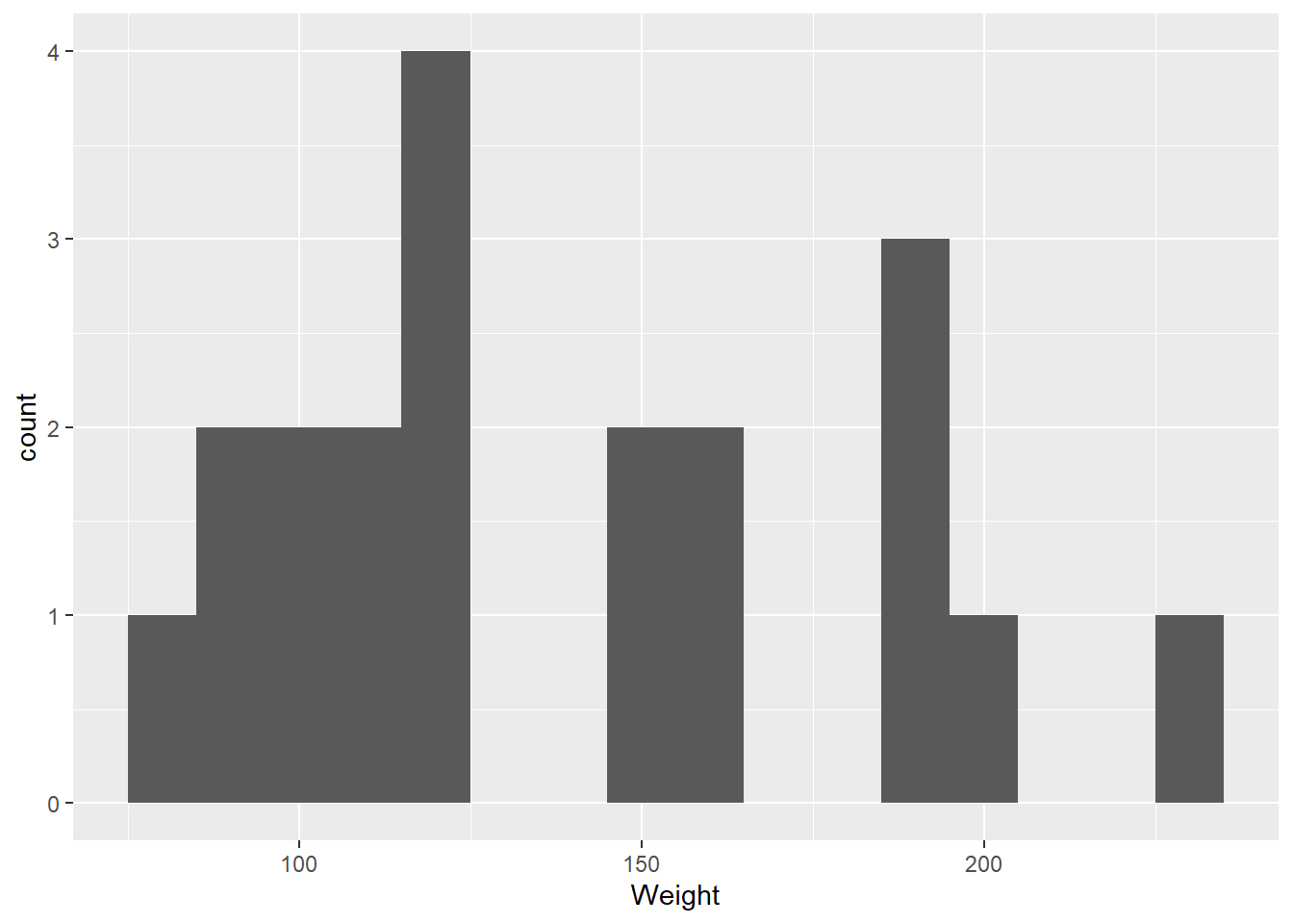
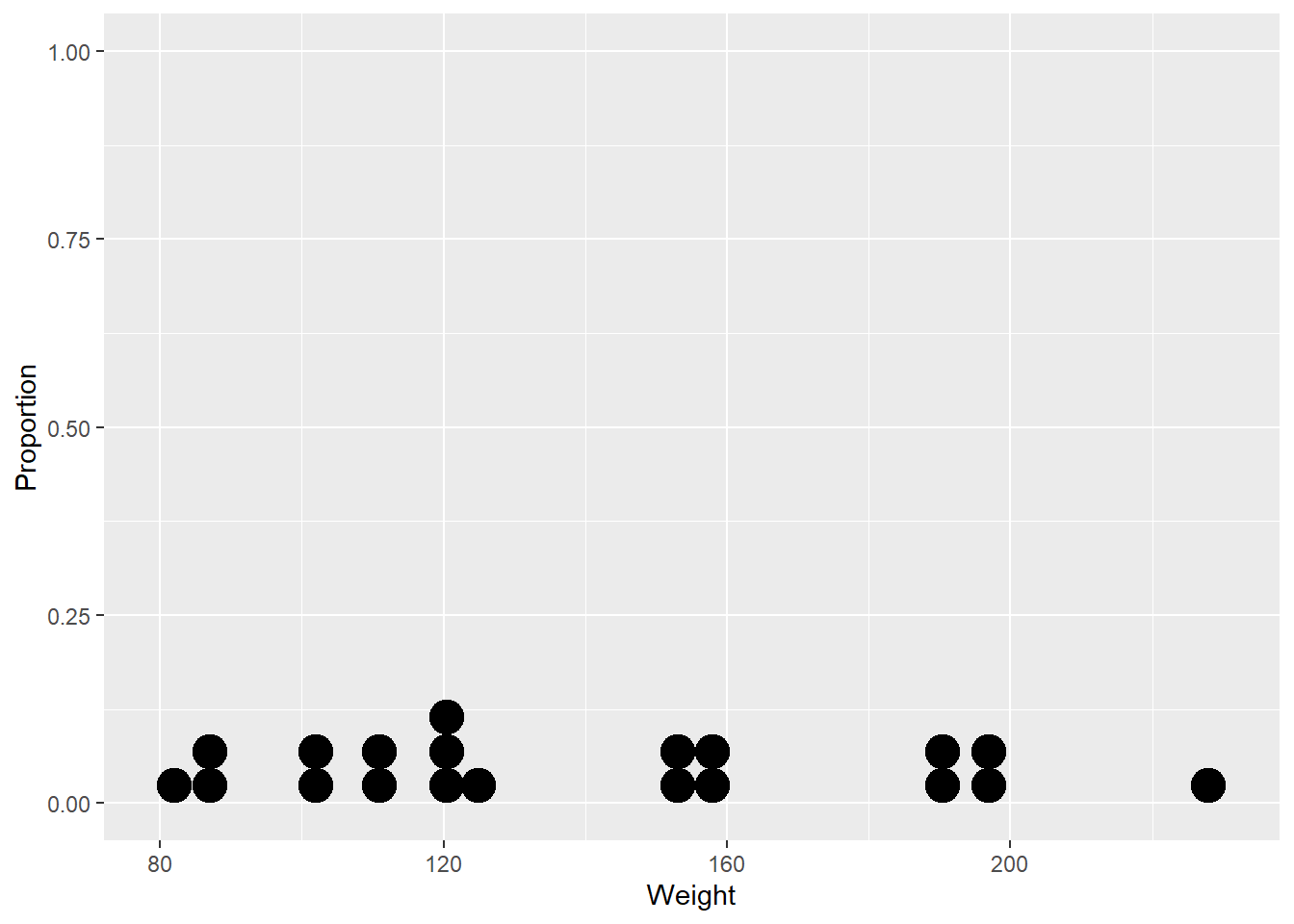
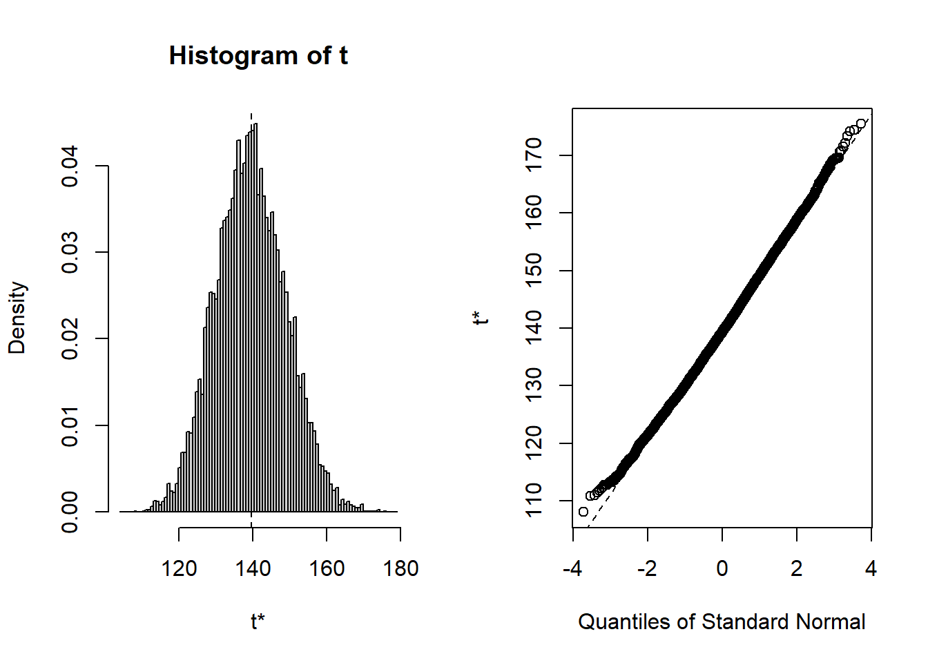
Consider the sample mean, \hat{\mu} = \sum_{i=1}^{n} X_i / n = \bar{X}. We can use the boot package to find the bootstrap distribution. We do so for the Weight data.
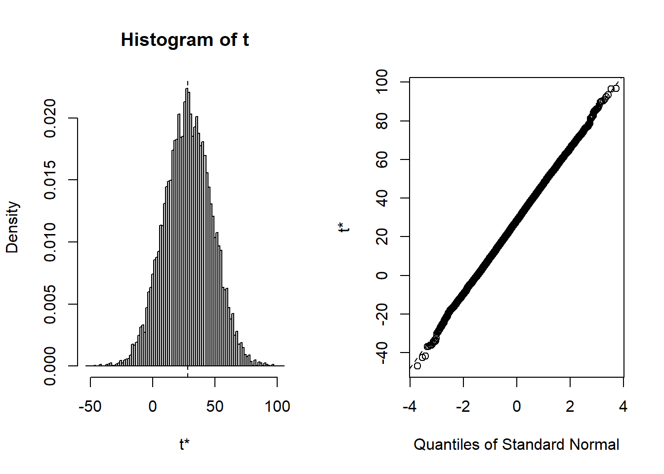
While the raw data appear to be non-normally distributed — abnormal? — the distribution of means seems to be normal. Apparently the Central Limit Theorem has kicked in. Note that the estimator appears to be unbiased. The standard error is estimated to be 9.444389. This is close to s/\sqrt{n}= 9.6423954. All of this is interesting and useful — later.
To get the bootstrap confidence interval, we use a quantile approach. We can trap a proportion of ``plausible’’ values between two values found by trimming the required percentages off of each end.
We see that a 95% CI for the mean is 121.7 to 158.3525 and a 99% CI for the mean is 116.45 to 164.5515.
The confidence intervals from above, and in particular the Percentile method, are similar to those given by the boot.ci function below.
Code
boot.ci(wt.mean.boot)
Warning in boot.ci(wt.mean.boot): bootstrap variances needed for studentized
intervals
BOOTSTRAP CONFIDENCE INTERVAL CALCULATIONS
Based on 9999 bootstrap replicates

CALL :
boot.ci(boot.out = wt.mean.boot)

Intervals :
Level      Normal              Basic
95%   (121.2, 158.2 )   (120.8, 157.5 )

Level     Percentile            BCa
95%   (121.7, 158.4 )   (122.6, 159.6 )
Calculations and Intervals on Original Scale
The Normal CI given above is calculated as \hat{\mu} \pm z_{(1-c)/2} {\text{se}}(\hat{\mu}) or \hat{\mu} \pm z_{\alpha/2} {\text{se}}(\hat{\mu}) where Z \sim {\text{N}}(0,1), c = 1-\alpha is the confidence level, and {\text{se}}(\hat{mu}) is the bootstrap standard error.
The Median
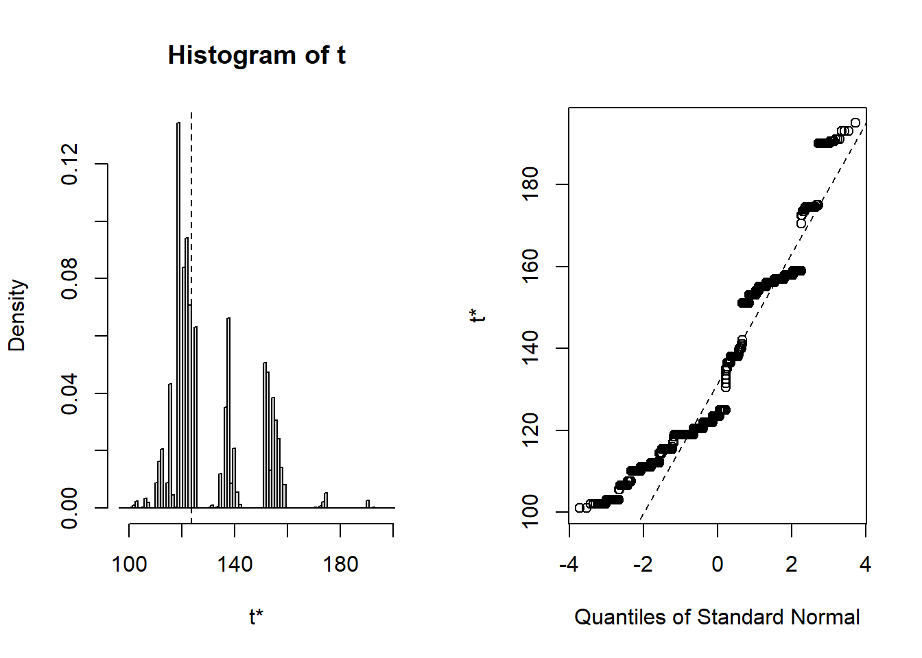
Consider the sample median, m, chosen such that P(X \le m)=P(X \ge m)=\frac{1}{2}. We can use the boot package to find the bootstrap distribution of the sample median. We do so using the Weight data from above.
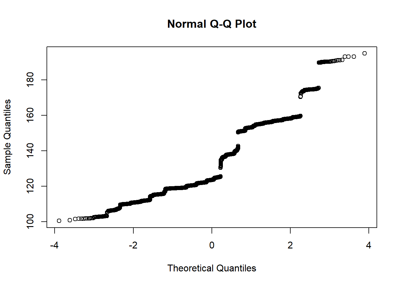
While the distribution of the bootstrap means seems to be normal, the distribution of the bootstrap medians does not. Since the Central Limit Theorem is a statement about the asymptotic distribution of sums of random variables (recalling the proof and the use of M_{\sum X_i}(t)), this should not be surprising. Note that the estimator appears to be biased. The standard error is estimated to be 15.847832.
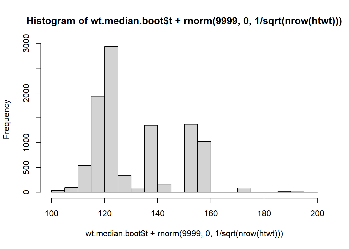
Because of the granularity of the bootstrap distribution we might be uncomfortable computing the bootstrap confidence interval for the median.
One suggested method for dealing with the granularity is to add a little random noise to smooth things out. Some authors suggest using \varepsilon \sim \text{N}\left(0, 1/n \right)
The confidence intervals computed above can be compared to those generated by boot.ci.
Code
boot.ci(wt.median.boot)
Warning in boot.ci(wt.median.boot): bootstrap variances needed for studentized
intervals
BOOTSTRAP CONFIDENCE INTERVAL CALCULATIONS
Based on 9999 bootstrap replicates

CALL :
boot.ci(boot.out = wt.median.boot)

Intervals :
Level      Normal              Basic
95%   ( 84.3, 146.4 )   ( 89.0, 136.0 )

Level     Percentile            BCa
95%   (111, 158 )   (110, 157 )
Calculations and Intervals on Original Scale
With an apparent lack of normality, it would be a waste of time to use a normal approach to computing a confidence interval.
Difference of Means
We can use the boot package to look at more interesting statistics. Consider creating a confidence interval for the difference of the means of two samples. As an example, we can look at the difference of GroupWeights using the data in the htwt data frame.
Code
wtgrp <- htwt[,c("Weight", "Group")] meanDiff <-function(x, i){### Compute group means y <-tapply(x[i,1], x[i,2], mean)### Return the difference y[1]-y[2] } wtgrp.meanDiff.boot <-boot(wtgrp, meanDiff, R=9999) wtgrp.meanDiff.boot
Warning in boot.ci(wtgrp.meanDiff.boot): bootstrap variances needed for
studentized intervals
BOOTSTRAP CONFIDENCE INTERVAL CALCULATIONS
Based on 9999 bootstrap replicates

CALL :
boot.ci(boot.out = wtgrp.meanDiff.boot)

Intervals :
Level      Normal              Basic
95%   (-9.47, 65.03 )   (-8.79, 65.05 )

Level     Percentile            BCa
95%   (-9.05, 64.79 )   (-9.79, 64.00 )
Calculations and Intervals on Original Scale
Normal and t Confidence Intervals
The bootstrap distribution of a statistic/estimator is supposed to resemble the sampling distribution of the same statistic/estimator. So, the distribution of the mean found above should be representative of what we would see if we sampled all possible samples of size n from the population.
We note that 95% of the sample means are within
Code
quantile(wt.mean.boot$t, c(0.025, 0.975))
    2.5%    97.5%
121.7000 158.3525
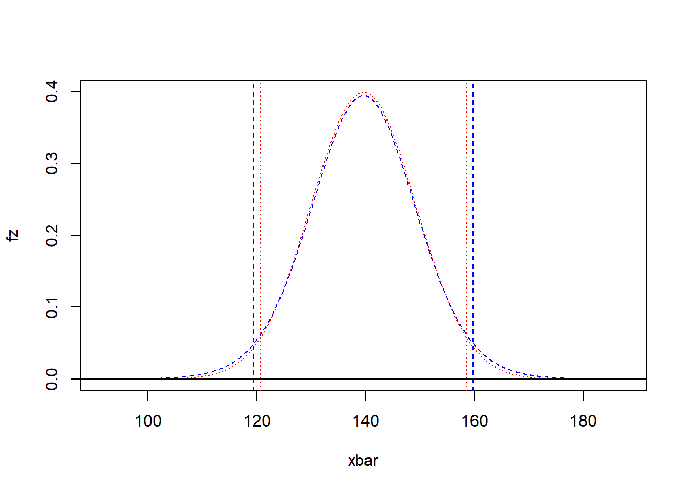
Assuming normality (which is supported by the plots generated above), the CLT suggests that the sample mean is distributed normally with mean, \mu = 139.6 and standard deviation s_{\bar{X}} = 43.1221/\sqrt{20} = 9.6423947. A plot of the normal (red/dot) and t (blue/dash) distributions for the weight data shows their differences.
So, 95.73% of the means are within 1.96 standard errors of \mu. We can turn this inside out and conclude that \mu is within 1.96 standard errors of 95.73% of the sample means. Hence, if we use \bar{X} \pm 1.96 \cdot \text{se}\left(\bar X\right) to create our intervals, 95% of the intervals will contain \mu.
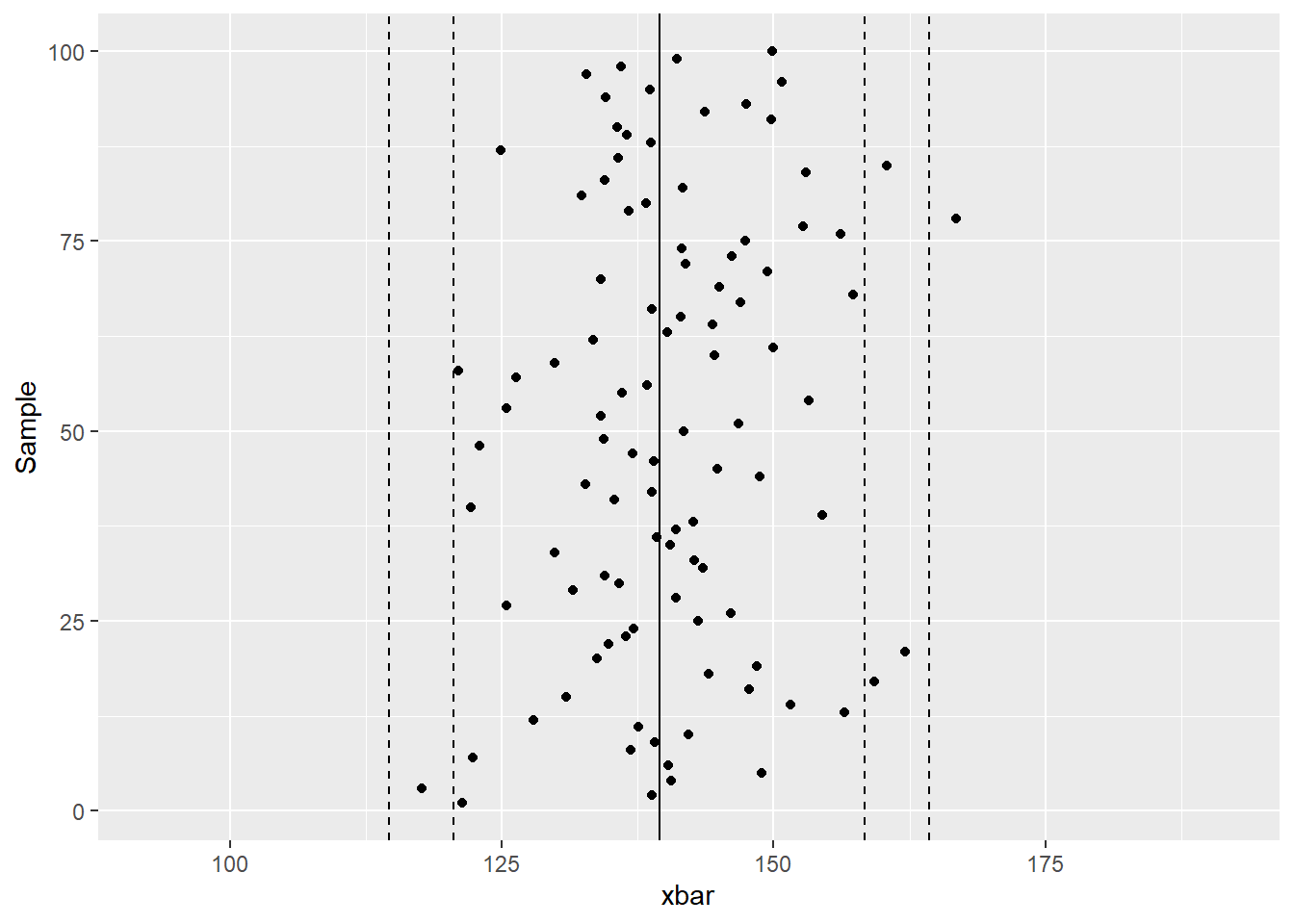
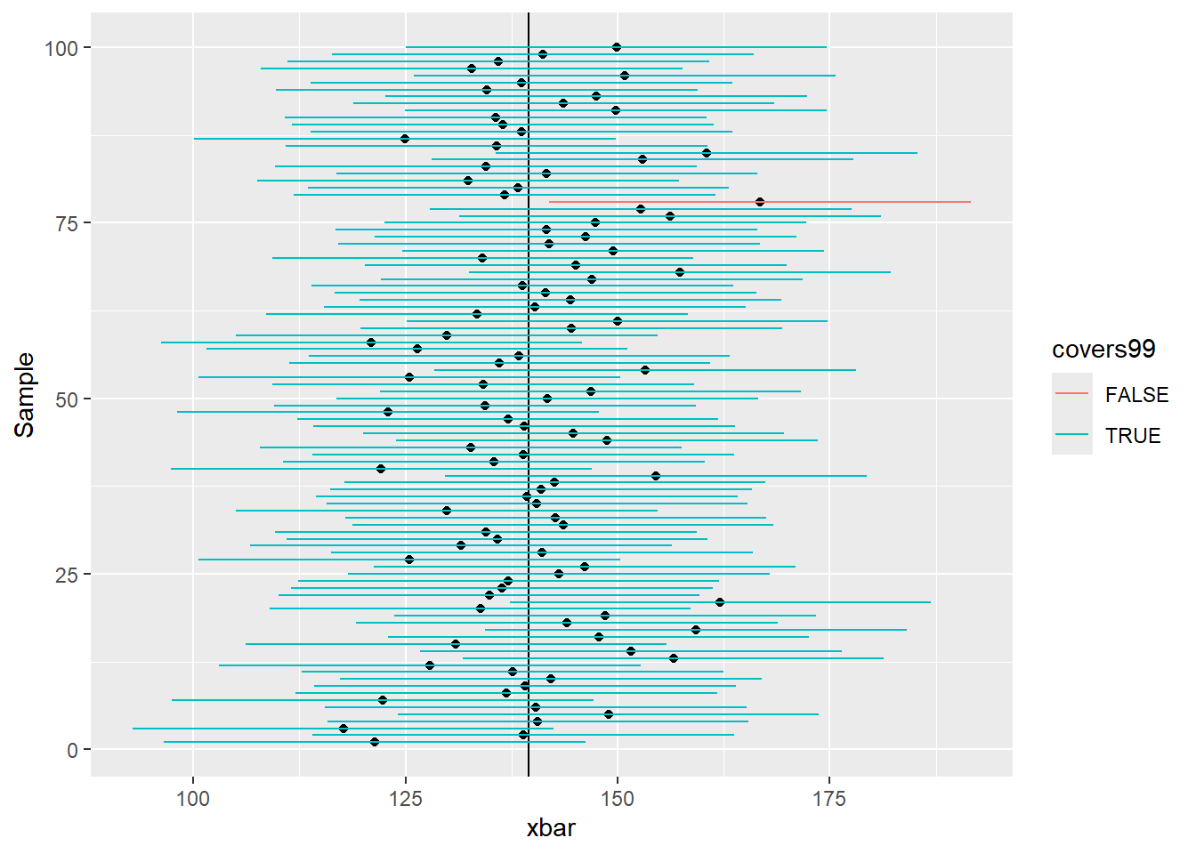
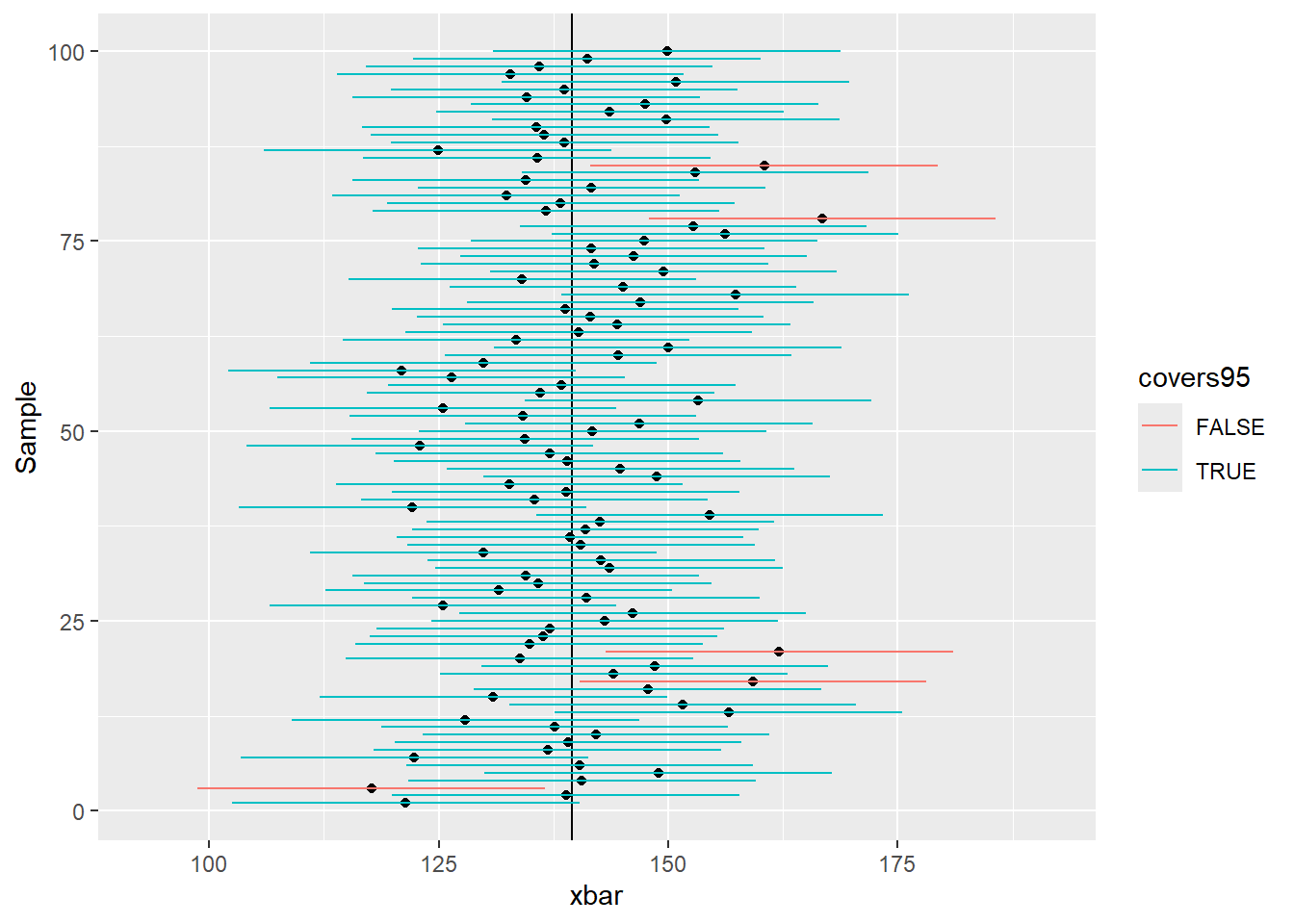
The plots below shows the proportion of means that fall within and outside of 95% and 99% CIs.
Code
seed <-47 nreps <-100 Sample <-1:nreps xbar <-sample(wt.mean.boot$t, nreps) mu <-mean(wt.mean.boot$t) l95 <- xbar -1.96* se u95 <- xbar +1.96* se l99 <- xbar -2.576* se u99 <- xbar +2.576* se covers95 <- l95 <= mu & mu <= u95 covers99 <- l99 <= mu & mu <= u99 df <-data.frame(Sample, l99, l95, xbar, u95, u99) p <-ggplot(df, aes(x=xbar, y=Sample)) +geom_point() +geom_vline(xintercept = mu) +xlim(range(c(l99,u99))) p +geom_vline(xintercept = mu +c(-2.576, -1.96, 1.96, 2.576)*se, lty=2)
Code
p +geom_segment(aes(x = l99, y = Sample, xend = u99, yend = Sample, color = covers99))
Code
p +geom_segment(aes(x = l95, y = Sample, xend = u95, yend = Sample, color = covers95))
To formalize this approach we note that above we used the bootstrap to generate percentile confidence intervals. We also used the bootstrap standard error to create normal confidence intervals for those bootstrap distributions that appeared to be normal.
It turns out that because of the CLT, when we know the population standard deviation, \sigma_X, we can still use the normal approximation for the mean and sum. In this case, the standard error of the mean is \sigma_{\bar{X}} = \sigma_x / \sqrt{n}. When the population standard deviation is not known, we can approximate it by using s_{\bar{X}} = s_x / \sqrt{n}. When we make this substitution, we also substitute a t-distribution (on n-1 degrees of freedom) for the normal.
Code
n <-length(htwt$Weight) s.xbar <-sqrt(var(htwt$Weight)/n) s.xbar
### Use the bootstrap std errormean(htwt$Weight) +qnorm(c(0.005, 0.025, 0.05, 0.95, 0.975, 0.995))*s.boot
Warning in qnorm(c(0.005, 0.025, 0.05, 0.95, 0.975, 0.995)) * s.boot: Recycling array of length 1 in vector-array arithmetic is deprecated.
  Use c() or as.vector() instead.
Warning in boot.ci(wt.mean.boot): bootstrap variances needed for studentized
intervals
BOOTSTRAP CONFIDENCE INTERVAL CALCULATIONS
Based on 9999 bootstrap replicates

CALL :
boot.ci(boot.out = wt.mean.boot)

Intervals :
Level      Normal              Basic
95%   (121.2, 158.2 )   (120.8, 157.5 )

Level     Percentile            BCa
95%   (121.7, 158.4 )   (122.6, 159.6 )
Calculations and Intervals on Original Scale
We see that the confidence intervals are slightly different. However, in this case, the differences are practically minimal — one or two pounds when looking at a mean of 139.6 pounds.
Theoretical CIs
The old-school, theoretical approach to creating confidence intervals is based upon the CDF and its inverse. In what follows, remember that the confidence level c is related to the hypothesis error type I error rate \alpha by c=1-\alpha.
Proportion
For the proportion, we note that each of the outcomes can be coded as a “success” or “failure”. This leads us to the use of X_i iid B(1,p) — or Bernoulli trials. The total number of “successes” is \sum_{i=1}^n X_i and \hat{p} = \bar{X}. Further, E\left(\bar{X}\right) = p and Var\left(\bar{X}\right) = p(1-p)/n.
By the CLT, for n “large” (variously np \ge 10andn(1-p) \ge 10, or np(1-p) \ge 5, etc.), \bar{X} \sim N\left(p, p(1-p)/n\right). To obtain a c = 1-\alpha level CI for p, we approximate the variance using \widehat{\sigma^2} = \hat{p}(1-\hat{p})/n and look at
\begin{align*}
1-\alpha & = P\left(z_{1-\alpha/2} \le \frac{\hat{p}-p}{\sqrt{\hat{p}(1-\hat{p})/n}} \le z_{\alpha/2} \right) \\
&= P\left(-\hat{p} + z_{1-\alpha/2}\sqrt{\hat{p}(1-\hat{p})/n} \le -p \le -\hat{p} + z_{\alpha/2}\sqrt{\hat{p}(1-\hat{p})/n} \right) \\
&= P\left(\hat{p} - z_{1-\alpha/2}\sqrt{\hat{p}(1-\hat{p})/n} \ge p \ge \hat{p} - z_{\alpha/2}\sqrt{\hat{p}(1-\hat{p})/n} \right) \\
&= P\left(\hat{p} - z_{\alpha/2}\sqrt{\hat{p}(1-\hat{p})/n} \le p \le \hat{p} + z_{\alpha/2}\sqrt{\hat{p}(1-\hat{p})/n} \right)
\end{align*}
Thus, an equal tailed c = 1-\alpha confidence interval for p is \hat{p} \pm z_{\alpha/2} \sqrt{\hat{p}(1-\hat{p})/n}.
Mean
For X_i iid E(X_i)=\mu and Var(X_i)=\sigma^2 the CLT indicates that when n is “large”, \bar{X} \sim N\left(\mu, \sigma^2/n\right). When \sigma^2 is known, and the X_i \sim N(\mu, \sigma^2) or n is large (n \ge 30), a c = 1-\alpha level CI for \mu can be computed as
\begin{align*}
1-\alpha & = P\left(z_{1-\alpha/2} \le \frac{\hat{\mu}-\mu}{\sigma/\sqrt{n}} \le z_{\alpha/2} \right) \\
&= P\left(-\hat{\mu} + z_{1-\alpha/2}\sigma/\sqrt{n} \le -\mu \le -\hat{\mu} + z_{\alpha/2}\sigma/\sqrt{n} \right) \\
&= P\left(\hat{\mu} - z_{1-\alpha/2}\sigma/\sqrt{n} \ge \mu \ge \hat{\mu} - z_{\alpha/2}\sigma/\sqrt{n} \right) \\
&= P\left(\hat{\mu} - z_{\alpha/2}\sigma/\sqrt{n} \le \mu \le \hat{\mu} + z_{\alpha/2}\sigma/\sqrt{n} \right)
\end{align*}
Thus, a symmetric, two-tailed c = 1-\alpha confidence interval for \mu is \bar{x} \pm z_{\alpha/2} \cdot \sigma/\sqrt{n}.
Variance
Recall that for X_i iid N(0,1), \sum_{i=1}^n X_i^2 \sim \chi^2_n. With a bit of hand waving (note that \bar{X} and s^2 are ancillary, etc.), we see that (n-1)s^2/\sigma^2 \sim \chi^2_{n-1}. Thus
\begin{align*}
1-\alpha & = P\left(\chi^2_{1-\alpha/2} < \frac{(n-1)s^2}{\sigma^2} < \chi^2_{\alpha/2}\right) \\
& = P\left(\frac{\chi^2_{1-\alpha/2}}{(n-1)s^2} < \frac{1}{\sigma^2} < \frac{\chi^2_{\alpha/2}}{(n-1)s^2}\right) \\
& = P\left(\frac{(n-1)s^2}{\chi^2_{1-\alpha/2}} < \sigma^2 < \frac{(n-1)s^2}{\chi^2_{\alpha/2}}\right)
\end{align*}
Thus, a two-tailed, c=1-\alpha confidence interval for \sigma^2 is
\left[\frac{(n-1)s^2}{\chi^2_{1-\alpha/2}},\frac{(n-1)s^2}{\chi^2_{\alpha/2}}\right]
Sample Size Estimation
Prior to collecting data one might be required to determine a sample size that will support a certain margin of error (me) at a certain confidence level. A guess for n can be made by noting that \text{me} = q^* \cdot \sigma_{\hat{\theta}} where q^* is some measure of confidence based on an appropriate distribution and \sigma_{\hat{\theta}} is the standard error of the estimator.
Mean
The appropriate sample size for a confidence interval for \mu when \sigma_X is known can be computed by recalling that \text{me} = z_{\alpha/2} \cdot \sigma_{\bar{X}}. We need only solve for n. Thus, we have
\text{me} = z_{\alpha/2} \cdot \frac{\sigma_X}{\sqrt{n}}
implies that we should choose n at least as large as
n = \left(\frac{z_{\alpha/2}\cdot\sigma_X}{\text{me}}\right)^2
Proportion
For the proportion, \hat{p}, recall that
\text{me} = z_{\alpha/2} \cdot \sqrt{\frac{p(1-p)}{n}}
Again, solving for n we get
n = \left(\frac{z_{\alpha/2} \cdot p(1-p)}{\text{me}}\right)^2
Unfortunately, p is unknown. Many statisticians plug in p=1/2 as this maximizes n. Others prefer to use \hat{p} from a prior study or they run a pilot study.