  x = 1:10
  x
[1] 1 2 3 4 5 6 7 8 9 10 ### Or
(x = 1:10) [1] 1 2 3 4 5 6 7 8 9 10 ### Or
print(x) [1] 1 2 3 4 5 6 7 8 9 10The theoretical distribution of the median is often not very friendly. To get a handle on what the distribution looks like for samples from different population distributions, we can use Efron’s bootstrap.
We will make ample use of the sample function. This function returns either a random subset of the original data, or a permutation — depending upon the number of items that you request it returns.
We first create a vector, x, that contains integers from 1 to 10.
x = 1:10
x [1] 1 2 3 4 5 6 7 8 9 10 ### Or
(x = 1:10) [1] 1 2 3 4 5 6 7 8 9 10 ### Or
print(x) [1] 1 2 3 4 5 6 7 8 9 10Now we sample, with and without replacement, from x. The results need not be stored.
  ### Get a random sample of size 5 from the n=10 w/o replacement
  sample(x, 5)
[1] 6 4 7 1 2 ### Get a random permutation of the n=10
sample(x) [1] 9 10 5 4 2 3 1 8 7 6 ### Get a bootstrap sample (of size n from the n=10 w/ replacement)
bootsamp = sample(x, replace = TRUE)
bootsamp [1] 1 10 2 7 9 8 1 4 6 10The default is to have each item have a selection probability of 1/n. We can specify other probabilities if we so choose.
  ### Creatae a boostrap sample from x with probabilities that favor the first five elements
  prob1 = c(rep(.15, 5), rep(.05, 5))
  rbind(x, prob1)
[,1] [,2] [,3] [,4] [,5] [,6] [,7] [,8] [,9] [,10]
x 1.00 2.00 3.00 4.00 5.00 6.00 7.00 8.00 9.00 10.00
prob1 0.15 0.15 0.15 0.15 0.15 0.05 0.05 0.05 0.05 0.05 sample(10, replace = TRUE, prob=prob1) [1] 7 1 1 3 7 9 1 3 6 2Sampling from a matrix is done similarly. We can sample from all elements of the matrix.
  ### Create a matrix filled with random values
  y1 = matrix( round(rnorm(25,5,2)), ncol=5)
  y1
[,1] [,2] [,3] [,4] [,5]
[1,] 4 5 5 4 3
[2,] 7 5 5 6 2
[3,] 3 2 8 6 7
[4,] 5 2 6 7 6
[5,] 4 5 8 5 7 ### Save a sample of size 5 in the vector x1
x1 = y1[sample(25, 5)]
x1[1] 5 2 3 4 2Or, we can sample entire rows.
  ### Create a matrix filled with random values
  y2 = matrix( round(rnorm(40, 5)), ncol=5)
  y2
[,1] [,2] [,3] [,4] [,5]
[1,] 6 4 5 4 6
[2,] 5 6 6 5 5
[3,] 5 7 5 6 6
[4,] 6 6 6 4 3
[5,] 5 4 6 4 7
[6,] 4 4 4 5 5
[7,] 6 6 6 6 4
[8,] 5 3 4 6 5 ### Save a sample of rows from y2 in the matrix x2
n = nrow(y2)
(i.rows = sample(n,3))[1] 7 3 8 x2 = y2[i.rows, ]
x2 [,1] [,2] [,3] [,4] [,5]
[1,] 6 6 6 6 4
[2,] 5 7 5 6 6
[3,] 5 3 4 6 5 ### More compactly
x2 = y2[sample(8, 3), ]
x2 [,1] [,2] [,3] [,4] [,5]
[1,] 4 4 4 5 5
[2,] 6 6 6 4 3
[3,] 6 6 6 6 4In the following example we find an estimate of the standard error for the estimate of the median. We will be using the lapply and sapply functions in combination with the sample function. (More information about the lapply and sapply functions can be found in the R help pages — help(“lapply”) or ?sapply in the console.)
Before we go on, let’s take a quick look at matrix computations. R allows us to apply a function to a dimension of a matrix — i.e. rows or columns. We apply the sum and mean functions to a matrix.
  ### Request the arguments for the matrix function
  args(matrix)
function (data = NA, nrow = 1, ncol = 1, byrow = FALSE, dimnames = NULL)
NULL ### Create a matrix of integers
x = matrix(1:16, nrow=4, byrow=TRUE)
x [,1] [,2] [,3] [,4]
[1,] 1 2 3 4
[2,] 5 6 7 8
[3,] 9 10 11 12
[4,] 13 14 15 16 ### Find the sum of all elements
sum(x)[1] 136 ### Find the row sums
args(apply)function (X, MARGIN, FUN, ..., simplify = TRUE)
NULL row.sums = apply(x, 1, sum)
cbind(x, row.sums) row.sums
[1,] 1 2 3 4 10
[2,] 5 6 7 8 26
[3,] 9 10 11 12 42
[4,] 13 14 15 16 58 ### Find the column sums
col.sums = apply(x, 2, sum)
rbind(x, col.sums) [,1] [,2] [,3] [,4]
1 2 3 4
5 6 7 8
9 10 11 12
13 14 15 16
col.sums 28 32 36 40 ### Total sum reprised
sum(x)[1] 136 sum(row.sums)[1] 136 sum(col.sums)[1] 136 ### And now for means
row.means = apply(x, 1, mean)
cbind(x, row.means) row.means
[1,] 1 2 3 4 2.5
[2,] 5 6 7 8 6.5
[3,] 9 10 11 12 10.5
[4,] 13 14 15 16 14.5 col.means = apply(x, 2, mean)
rbind(x, col.means) [,1] [,2] [,3] [,4]
1 2 3 4
5 6 7 8
9 10 11 12
13 14 15 16
col.means 7 8 9 10 mean(row.means)[1] 8.5 mean(col.means)[1] 8.5 mean(x)[1] 8.5Of course, all of the above could have been computed using matrix/vector operations.
dim(x)[1] 4 4 n = length(x)
n.row = n.col = nrow(x)
(ones = rep(1, n.row))[1] 1 1 1 1 ones %*% x [,1] [,2] [,3] [,4]
[1,] 28 32 36 40 x %*% ones [,1]
[1,] 10
[2,] 26
[3,] 42
[4,] 58 ones %*% x %*% ones [,1]
[1,] 136 ones %*% x / n.col [,1] [,2] [,3] [,4]
[1,] 7 8 9 10 x %*% ones / n.row [,1]
[1,] 2.5
[2,] 6.5
[3,] 10.5
[4,] 14.5 ones %*% x %*% ones / n [,1]
[1,] 8.5We return to using the bootstrap to model the sampling distributions of a statistic.
  ### Create a data set by taking 100 random observations from a normal
  ### distribution with mean 5 and stdev 3. Each observation has been
  ### rounded to the nearest integer.
  data <- round(rnorm(100, 5, 3))

  ### Display the first ten observations
  data[1:10]
[1] 5 8 5 3 10 7 3 -1 6 5The lapply function applies a given function to a list by passing the list elements to the function. We use lapply to run a function that generates a sample of the same size as the original sample by sampling with replacement.
  ### Generate n.boots bootstrap samples. Note that the function has an argument i
  ### that is not passed to the sample function which uses the global
  ### data instead.
  n.boots = 9999
  resamples = lapply(1:n.boots, function(i) sample(data, replace = T))

  ### Display the results for the third resample --- the others are similar.
  resamples[3]
[[1]]
[1] 5 5 5 10 1 10 1 8 4 4 8 -1 11 3 2 11 5 10 -1 11 6 6 8 7 11
[26] 5 -2 3 4 7 2 4 7 4 7 7 3 3 9 7 5 9 2 4 5 9 10 6 11 5
[51] 6 3 10 5 10 4 4 1 3 5 9 1 8 6 -1 6 4 6 7 7 3 4 6 9 1
[76] 11 5 5 8 -1 4 6 5 6 4 2 7 1 11 3 5 8 1 8 7 9 7 7 0 7We can now apply the median function to each of the bootstrap samples to generate a bootstrap distribution.
  ### Calculate the median for each bootstrap sample
  r.median <- sapply(resamples, median)
  r.median[1:15]  ### Look at 15 of these
[1] 5 6 5 5 5 6 5 5 6 4 5 5 5 5 6 ### Compute summary statistics for the distribution of the medians
summary(r.median) Min. 1st Qu. Median Mean 3rd Qu. Max.
3.500 5.000 5.000 5.161 5.000 7.000 ### Display a histogram of the distribution of the medians
hist(r.median)
abline(v=mean(data), lty=3)
abline(v=mean(r.median), lty=1)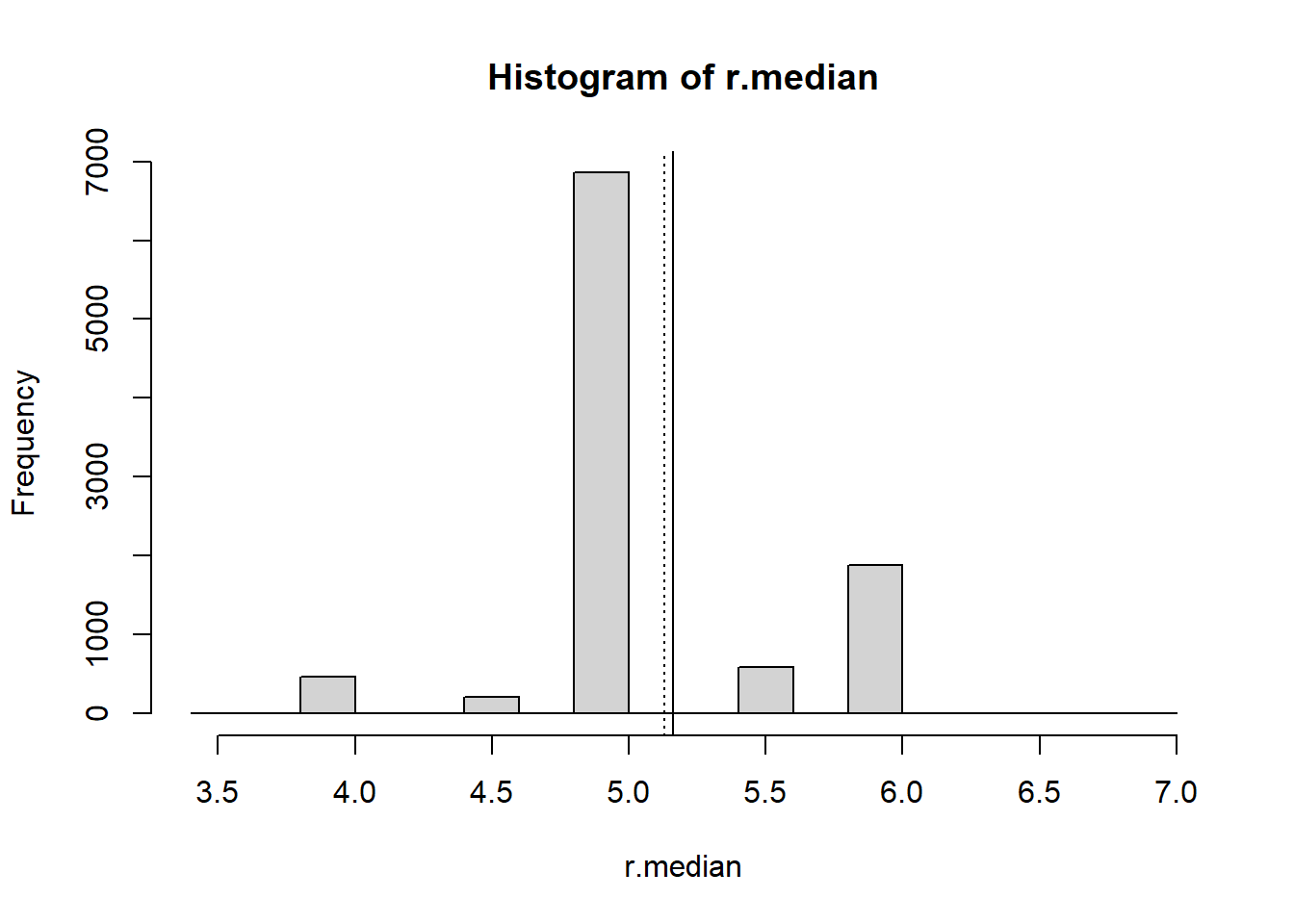
  ### Display a normal probability plot
  qqnorm(r.median)
  qqline(r.median)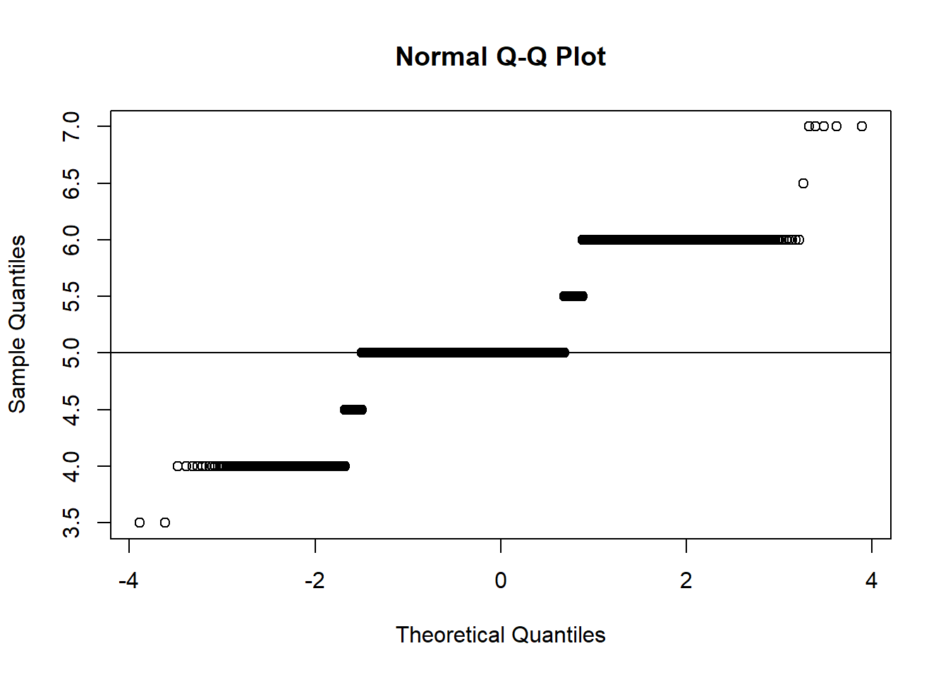
  ### Display a quantile-quantile plot using a standard normal
  n = length(r.median)
  qqplot(qnorm(ppoints(n)), r.median,
       main = "Q-Q plot for Normal")
  qqline(r.median, distribution = function(p){qnorm(p)},
       probs = c(0.25, 0.75), col = 2)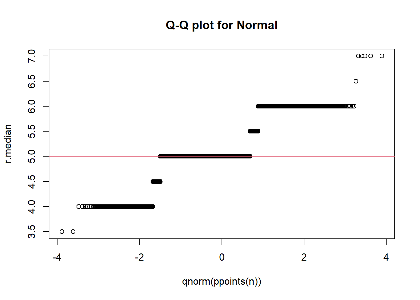
  ### Display a quantile-quantile plot using a chiquare
  n = length(r.median)
  qqplot(qchisq(ppoints(n), df = n-1), r.median,
       main = expression("Q-Q plot for" ~~ {chi^2}[nu == n-1]))
  qqline(r.median, qtype = 5, distribution = function(p){qchisq(p, df = n-1)},
       probs = c(0.1, 0.6), col = 2)
  mtext("qqline(*, dist = qchisq(., df=n-1), prob = c(0.1, 0.6))")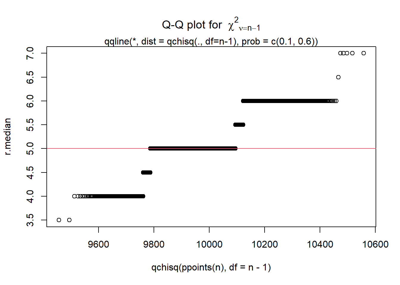
These steps can be combined into a single function where all we would need to specify is which data set to use and how many times we want to resample in order to obtain the adjusted standard error of the median.
  ### Function to bootstrap the mean, standard error, and bias of the median
  b.median = function(data, nboot=9999) {
    resamples = lapply(1:nboot, function(i) sample(data, replace=T))
    r.median = sapply(resamples, median)
    d.xbar = mean(data)
    r.xbar = mean(r.median)
    r.bias = r.xbar - d.xbar
    r.stderr = sqrt(var(r.median))
    list(xbar=r.xbar, std.err=r.stderr, bias=r.bias, resamples=resamples,
         medians=r.median
        )
  }

  ### Create some data to be used (same as in the above example)
  data1 = round(rnorm(100, 5, 3))

  ### Save the results of 10000 boots of the function b.median in the object b1
  b1 = b.median(data1, 10000)

  ### Display the third of the 10000 bootstrap samples
  b1$resamples[3]
[[1]]
[1] 7 -1 8 5 6 9 5 3 6 4 6 5 5 4 5 7 2 9 7 9 8 10 4 7 8
[26] -1 3 8 2 6 7 6 8 6 2 4 6 0 4 8 2 4 6 7 2 0 9 6 -2 1
[51] 5 6 9 4 6 -2 4 2 4 6 14 6 2 4 -1 8 7 4 1 11 -1 3 5 6 2
[76] 7 7 6 5 4 10 3 5 11 6 4 4 6 1 -1 4 1 1 1 0 4 7 2 -2 4 ### Display the mean, standard error, and bias of bootstrapped medians
print(c(b1$xbar, b1$std.err, b1$bias))[1] 5.2015000 0.5482954 0.0715000 ### Display a histogram of the distribution of medians
hist(b1$medians)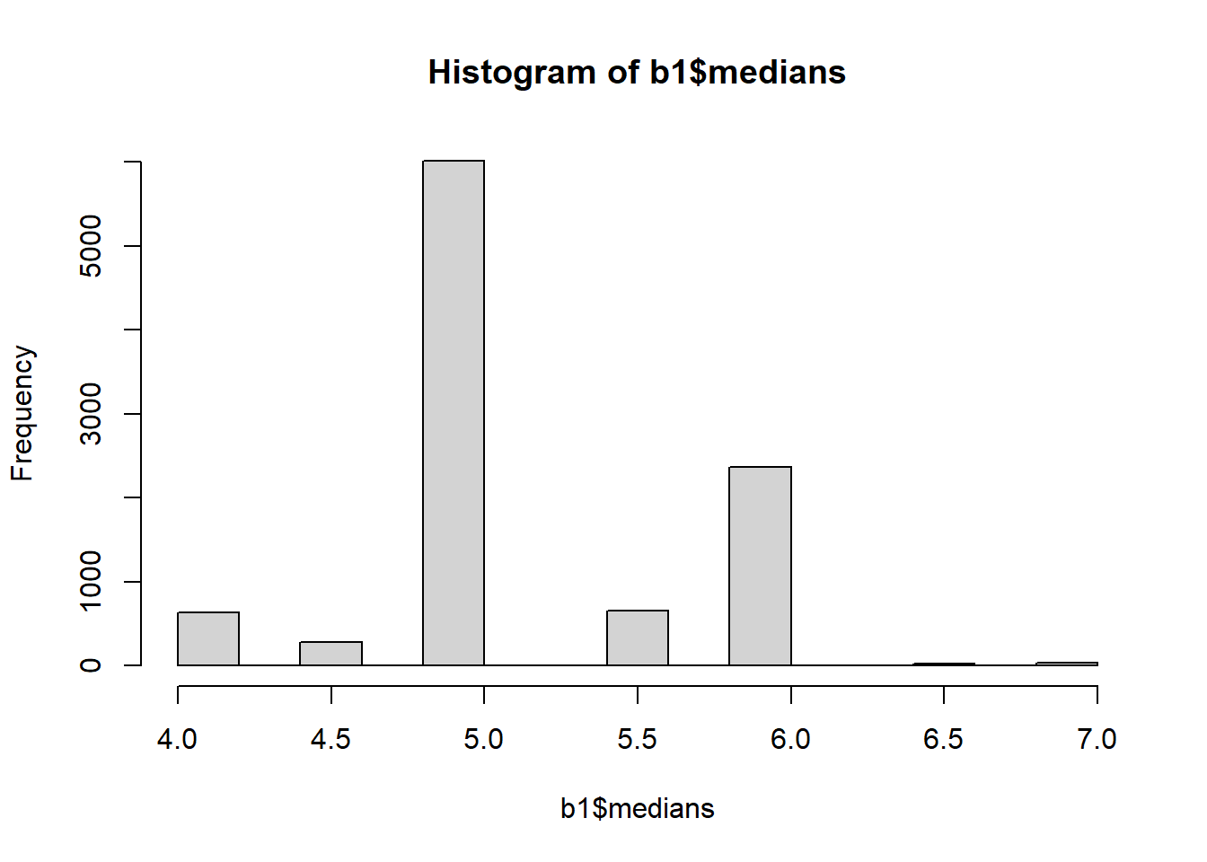
  ### Make a normal probability plot
  qqnorm(b1$medians)
  qqline(b1$medians)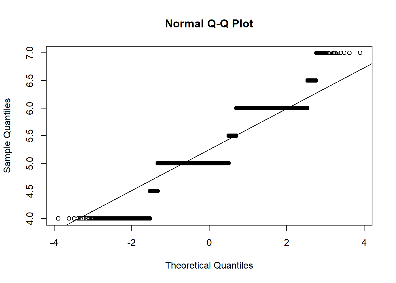
qqPlot(b1$medians)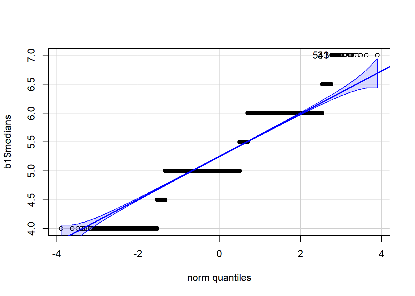
[1] 31 543 ### We can input the data directly into the function and display
### the standard error in one line of code.
b.median(data1)$std.err[1] 0.5479893 ### Or, we can make the histogram in one line
hist(b.median(data1)$medians)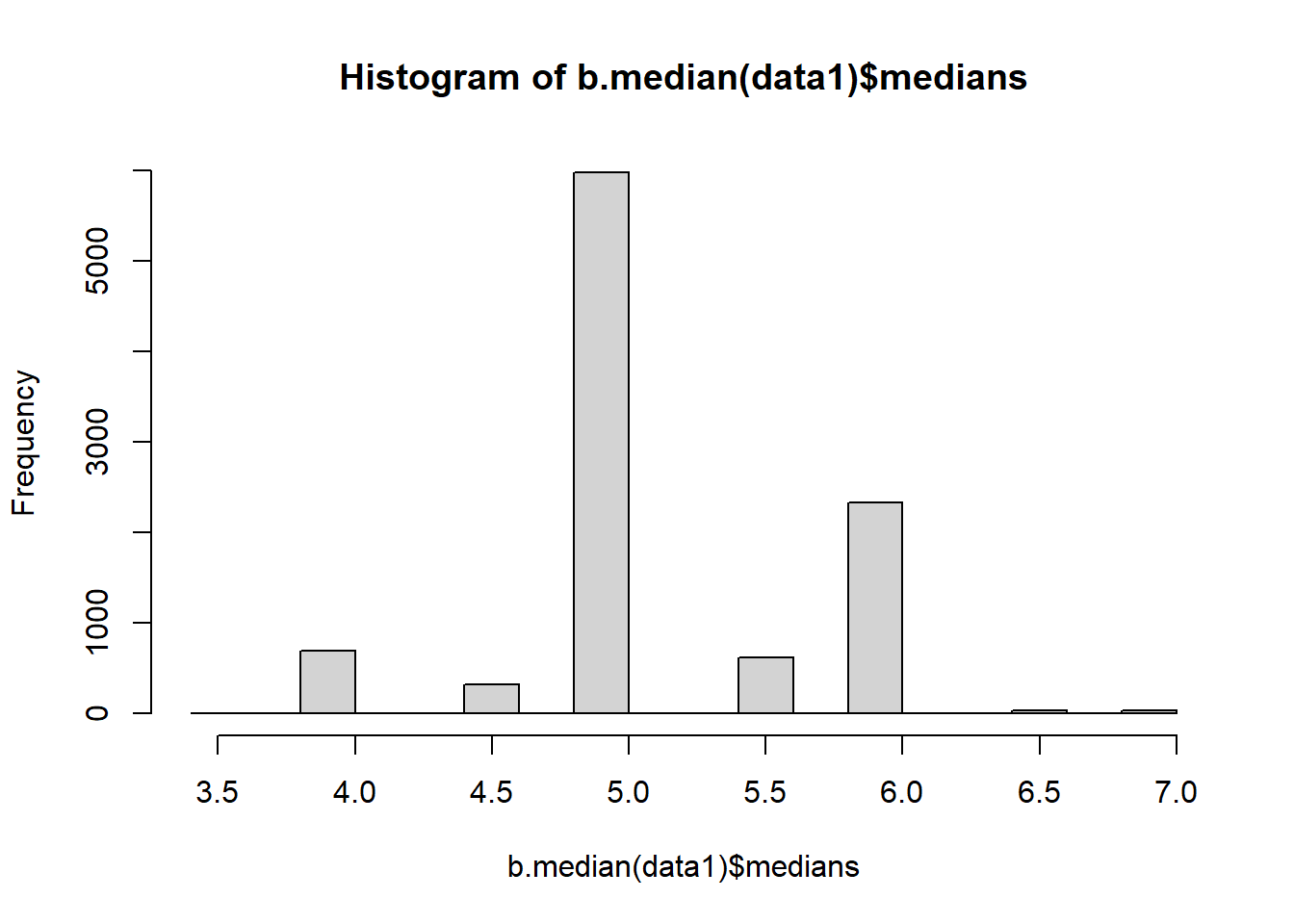
Note that the single line calls generate plots based upon different bootstrap samples. This approach is also not very time efficient.
It would be fairly simple to generalize the function to work for any summary statistic. We show this approach for the sample mean.
  ### Function to bootstrap the mean, standard error, and bias of a statistic
  b.stat = function(data, nboot=9999, fnct = mean, ...) {
    resamples = lapply(1:nboot, function(i) sample(data, replace=T))
    r.boots = sapply(resamples, fnct, ...)
    d.xbar = mean(data)
    r.xbar = mean(r.boots)
    r.bias = r.xbar - d.xbar
    r.stderr = sqrt(var(r.boots))
    list(xbar=r.xbar, std.err=r.stderr, bias=r.bias, resamples=resamples,
         boots=r.boots
        )
  }

  ### Reuse the data created above so that we can compare mean and median
  ### Save the results of 10000 boots of the function b.median in the object b2
  b2 = b.stat(data1, 9999, function(x){mean(x)})

  ### Display the third of the 10000 bootstrap samples
  b2$resamples[3]
[[1]]
[1] 7 6 9 7 2 4 4 2 1 2 0 0 0 4 7 7 4 4 1 4 7 1 4 2 5
[26] 3 6 5 9 2 6 6 6 3 3 9 3 1 -2 8 1 4 8 0 1 5 7 4 -1 6
[51] 9 10 10 11 9 4 12 7 8 3 7 5 6 7 -2 8 5 2 3 7 7 4 4 9 -1
[76] 7 8 3 3 4 11 5 0 7 4 7 7 8 0 2 3 6 8 6 2 5 8 6 9 1 ### Display the mean, standard error, and bias of bootstrapped means
print(round(c(b2$xbar, b2$std.err, b2$bias), 4))[1] 5.1242 0.3244 -0.0058 ### Display a histogram of the distribution of means
hist(b2$boots)
abline(v = b2$xbar, lty = 1)
abline(v = mean(data1), lty = 3)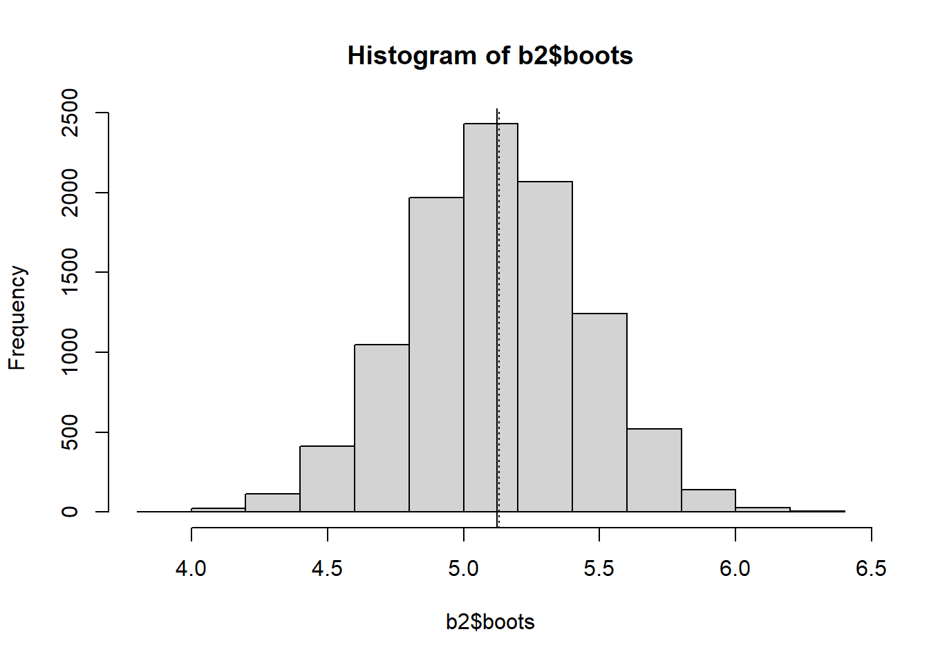
  ### Make a normal probability plot
  qqnorm(b2$boots)
  qqline(b2$boots)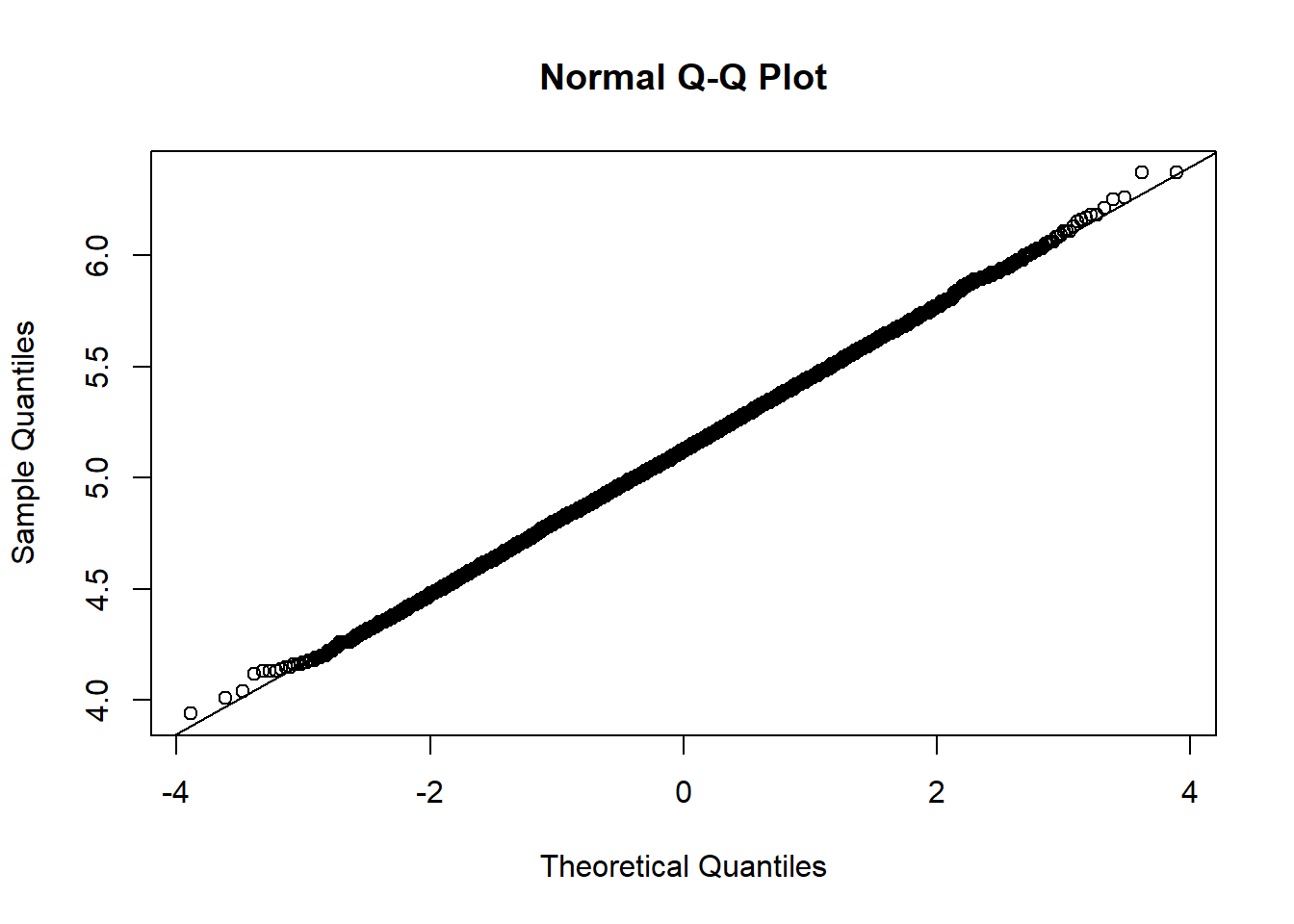
qqPlot(b2$boots)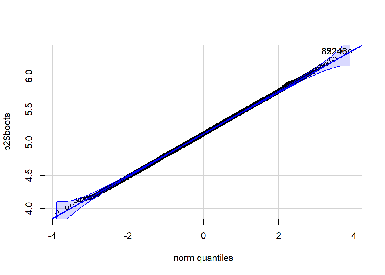
[1] 822 5246There exists a package, boot, that already has a bootstrapping function that acts like the function that we created in the code chunk above. The advantage of using boot is that it has some additional methods of doing things.
  ### Bootstrap of the median of the data1 data from above.
  ### Make sure that the boot package is installed using
  ### install.packages("boot"), or use a package like pacman to take care
  ### of installation and loading.
  #library(boot)
  p_load(boot)

  ### Define the median function with data, d, and boot sample indices, i.
  mystat = function(d, i){
                           median(d[i])
                          }

  ### Use the boot function to run the bootstrap
  b3 = boot(data1, mystat, R=9999)
  b3
ORDINARY NONPARAMETRIC BOOTSTRAP


Call:
boot(data = data1, statistic = mystat, R = 9999)


Bootstrap Statistics :
    original    bias    std. error
t1* 5 0.2014201 0.5512665 plot(b3)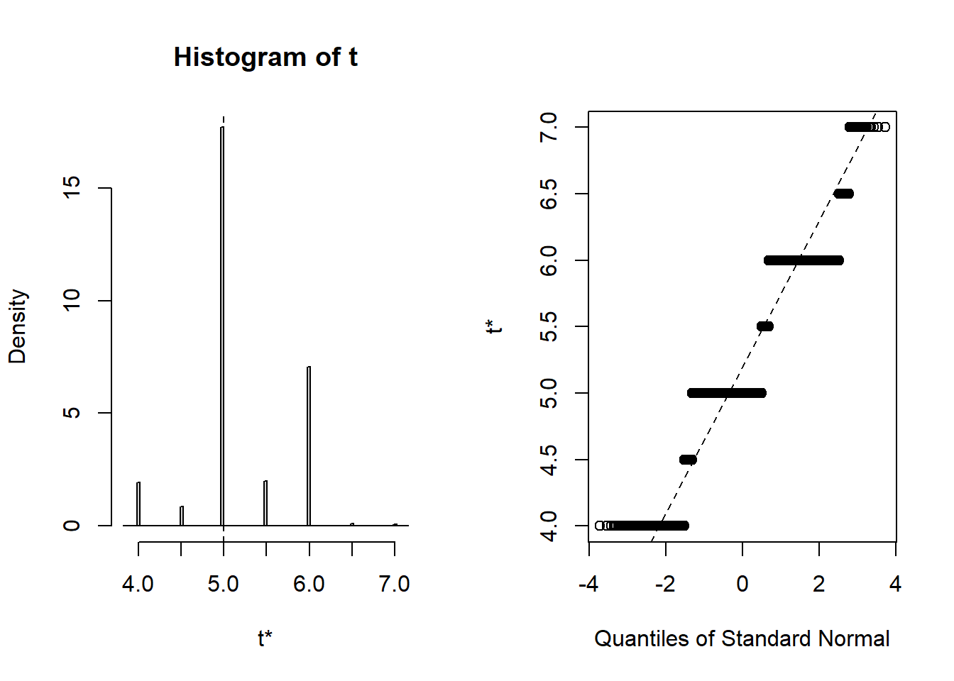
  ### Display a quantile-quantile plot using a chiquare
  b3$t[1:15]  ### The boot statistics are stored in a variable, t, within the the boot object.
[1] 5.0 6.0 5.0 5.5 5.0 5.0 5.0 5.0 5.0 5.0 6.0 5.0 5.0 5.0 5.0 n = length(b3$t)
qqplot(qchisq(ppoints(n), df = n-1), b3$t,
main = expression("Q-Q plot for" ~~ {chi^2}[nu == n-1]))
qqline(b3$t, qtype = 5, distribution = function(p){qchisq(p, df = n-1)},
probs = c(0.1, 0.6), col = 2)
mtext("qqline(*, dist = qchisq(., df=n-1), prob = c(0.1, 0.6))")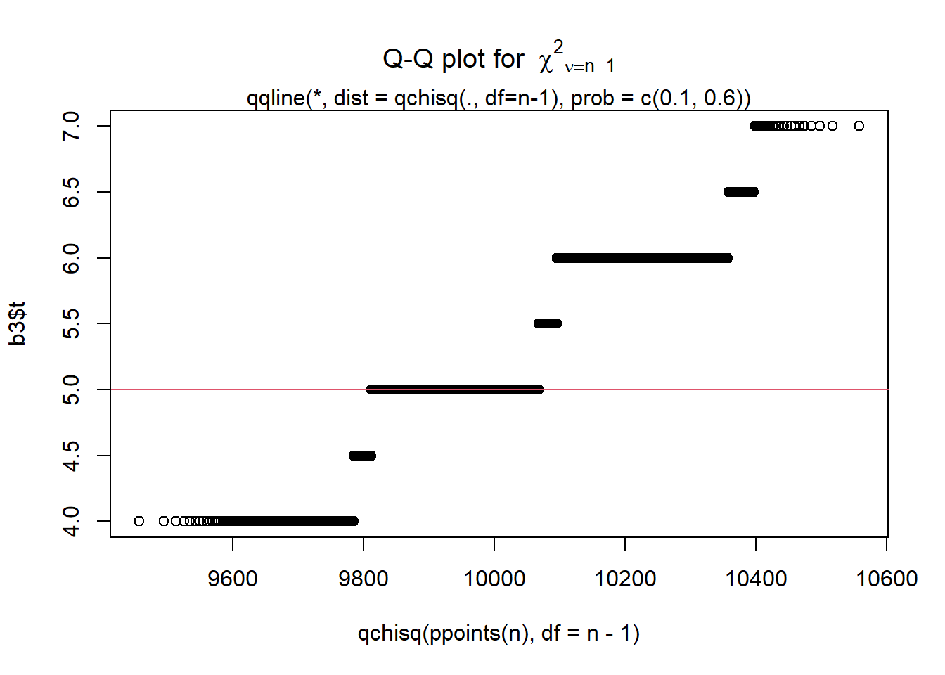
qqPlot(b3$t, distribution="chisq", df=n-1)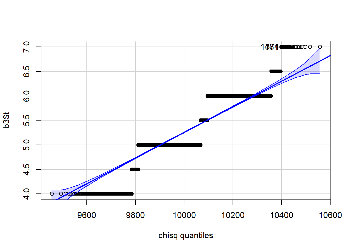
[1] 481 1374More complex statistics can be bootstrapped. We look at the mean ratio of weight to height for college students.
  ### Get the data
  htwt = read.csv("http://facweb1.redlands.edu/fac/jim_bentley/downloads/math111/htwt.csv")
  head(htwt)
Height Weight Group
1 64 159 1
2 63 155 2
3 67 157 2
4 60 125 1
5 52 103 2
6 58 122 2 ### Usual bootstrap of the ratio of means
ratio = function(d, i){ mean(d$Weight[i] / d$Height[i]) }
b4 = boot(htwt, ratio, R = 9999)
b4
ORDINARY NONPARAMETRIC BOOTSTRAP


Call:
boot(data = htwt, statistic = ratio, R = 9999)


Bootstrap Statistics :
    original       bias    std. error
t1* 2.20046 -0.002444086 0.08457255 plot(b4)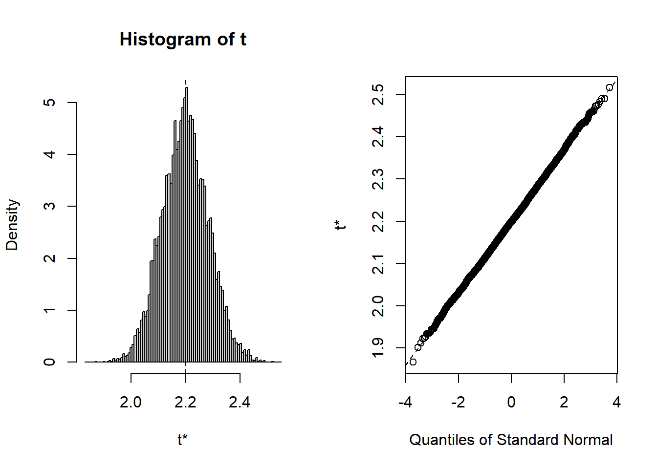
  ### Display a quantile-quantile plot using a gamma --- which it probably isn't
  b4$t[1:15]  ### The boot statistics are stored in a variable, t, within the the boot object.
[1] 2.076479 2.224253 2.369241 2.214466 2.135009 2.203942 2.318061 2.230058
[9] 2.210810 2.167490 2.271731 2.195071 2.256139 2.285043 2.260207 n = length(b4$t)
s = var(b4$t)/mean(b4$t) ### Estimate the scale parameter
a = mean(b4$t)/s ### Estimate the shape
qqplot(qgamma(ppoints(n), shape = a, scale = s), b4$t,
main = paste0("Q-Q plot for Gamma(shape = ", round(a,2), ", scale = ", round(s,4), ")")
)
qqline(b4$t, qtype = 5, distribution = function(p){qgamma(p, shape = a, scale = s)},
probs = c(0.1, 0.6), col = 2)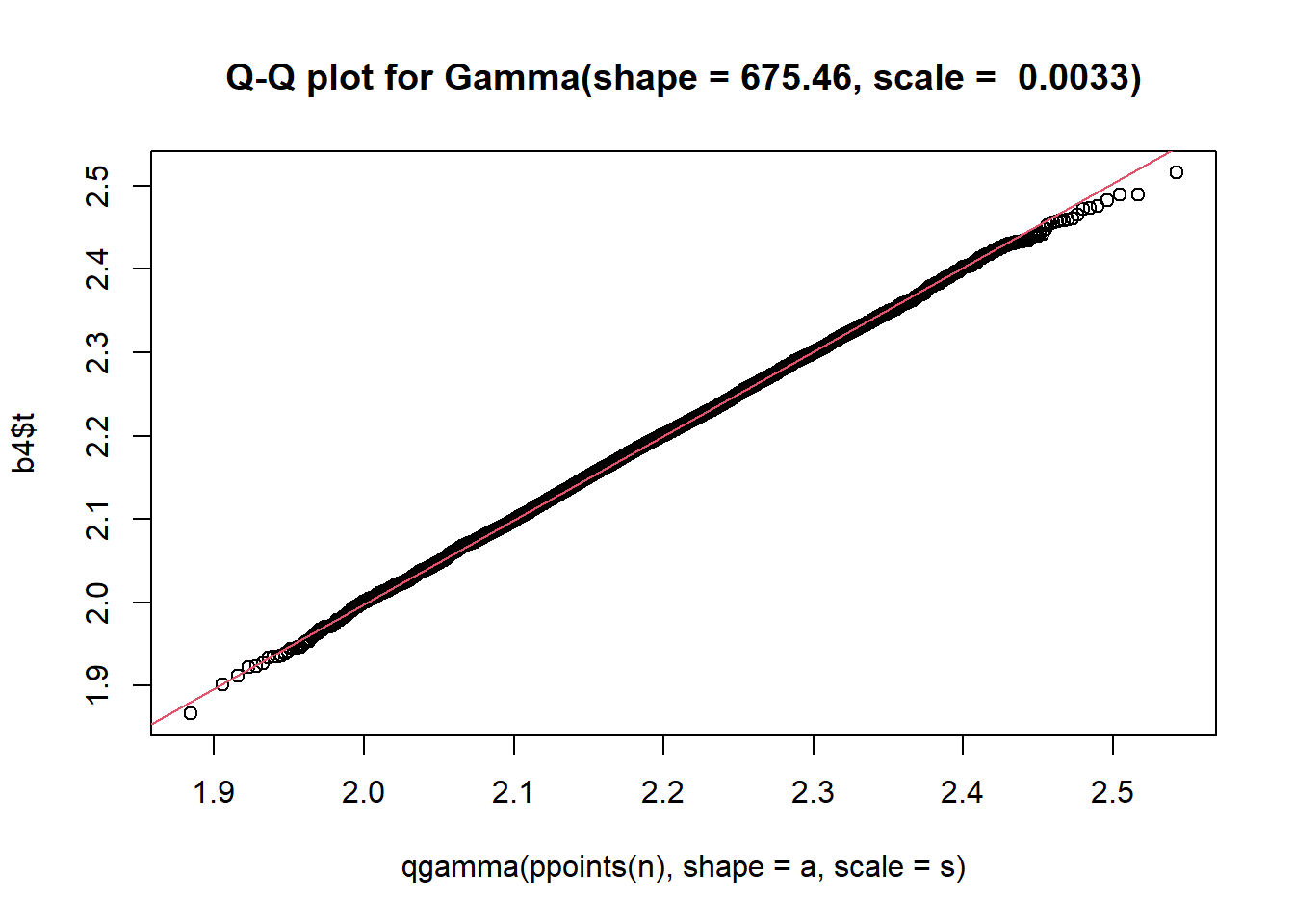
qqPlot(b4$t, distribution="gamma", shape=a, scale=s)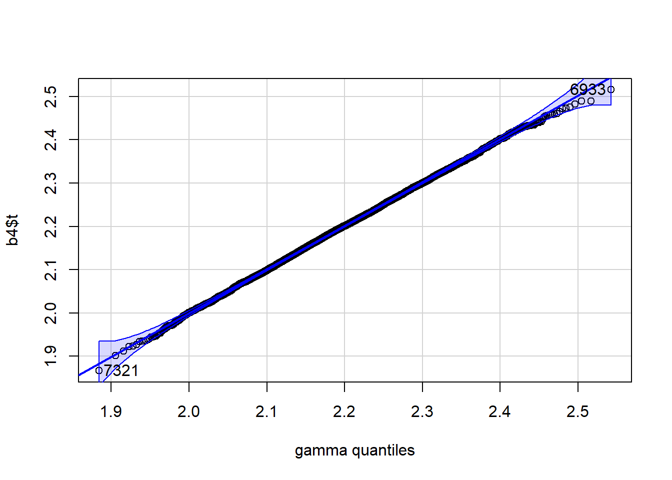
[1] 7321 6933 ### Using base R
x = rnorm(100,10,5)
qqnorm(x)
qqline(x)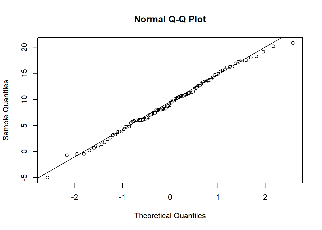
  p_load(car)

  qqPlot(x=rnorm(100,10,5))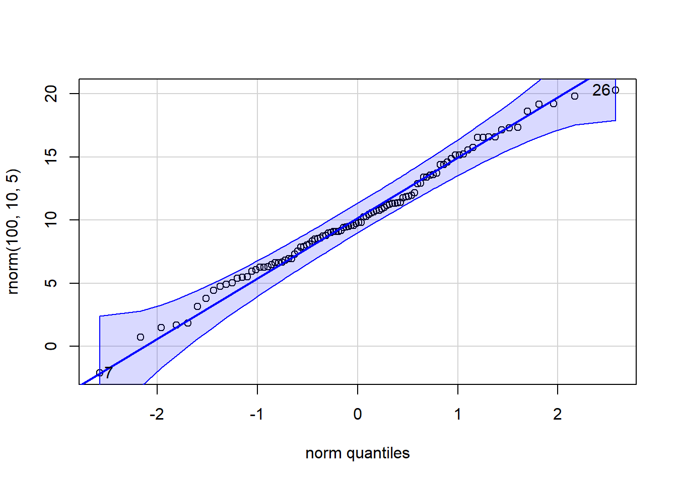
[1] 7 26 qqPlot(x=rnorm(100,10,5), distribution="chisq", df=5)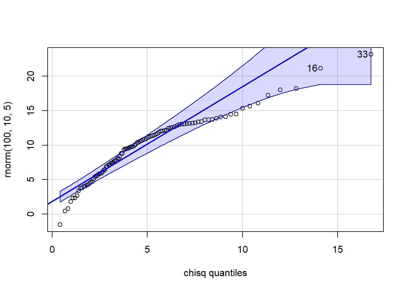
[1] 33 16 qqPlot(x=rchisq(100,5), distribution="chisq", df=25)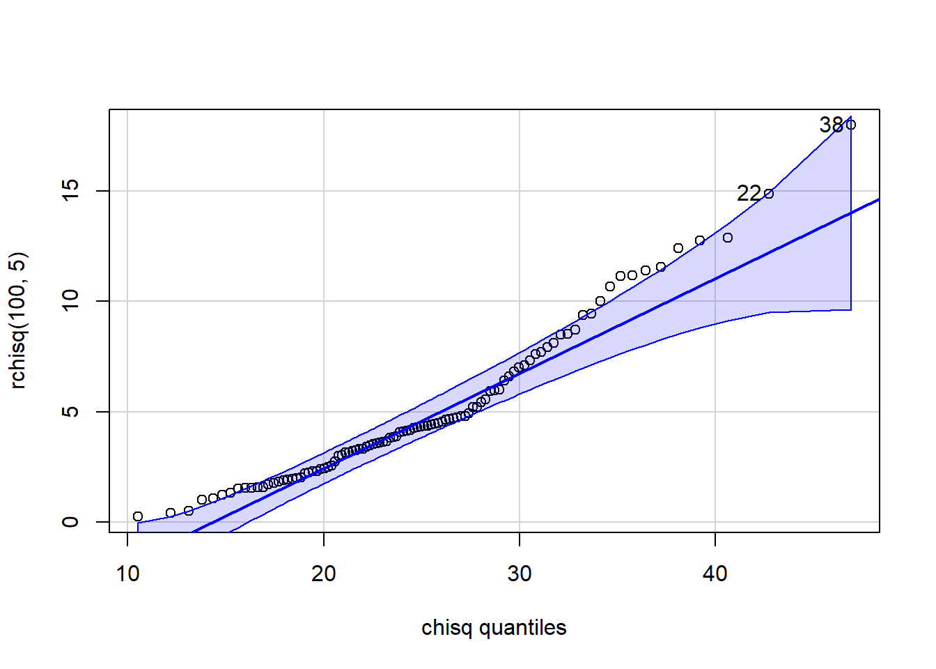
[1] 38 22 qqPlot(x=rchisq(100,5), distribution="chisq", df=5)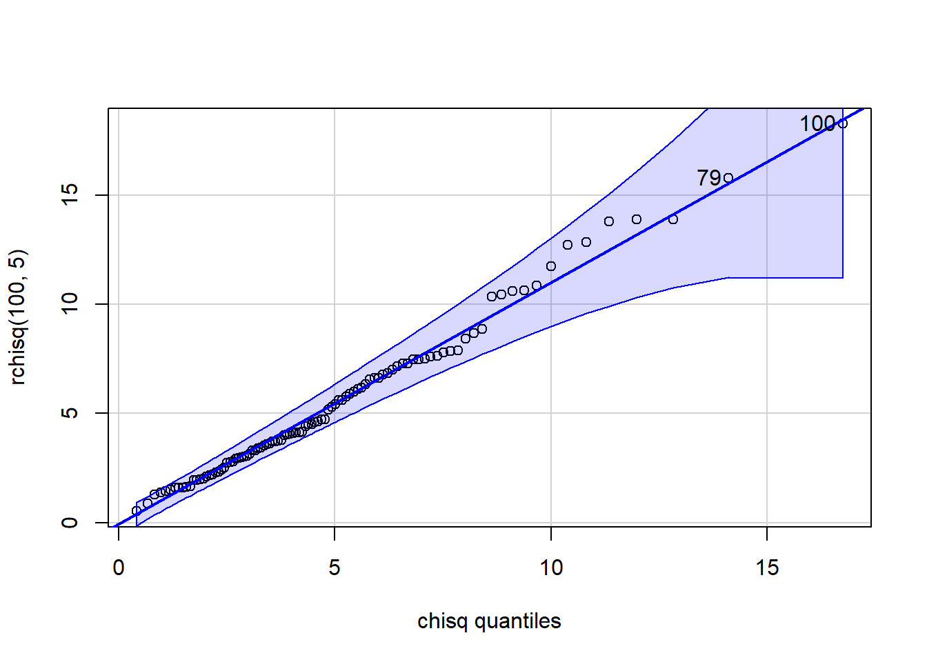
[1] 100 79 p_load(ggplot2)
p_load(qqplotr)
p_load(dplyr) ### Needed for piping and tibble creation
tibble(x = rnorm(100,10,5)) %>%
ggplot(aes(sample = x)) +
stat_qq_band(bandType = "pointwise", fill = "#8DA0CB", alpha = 0.4) +
stat_qq_line(colour = "#8DA0CB") +
stat_qq_point() +
ggtitle("Normal") +
xlab("Normal quantiles") +
ylab("rnorm(100,10,5") +
theme_light()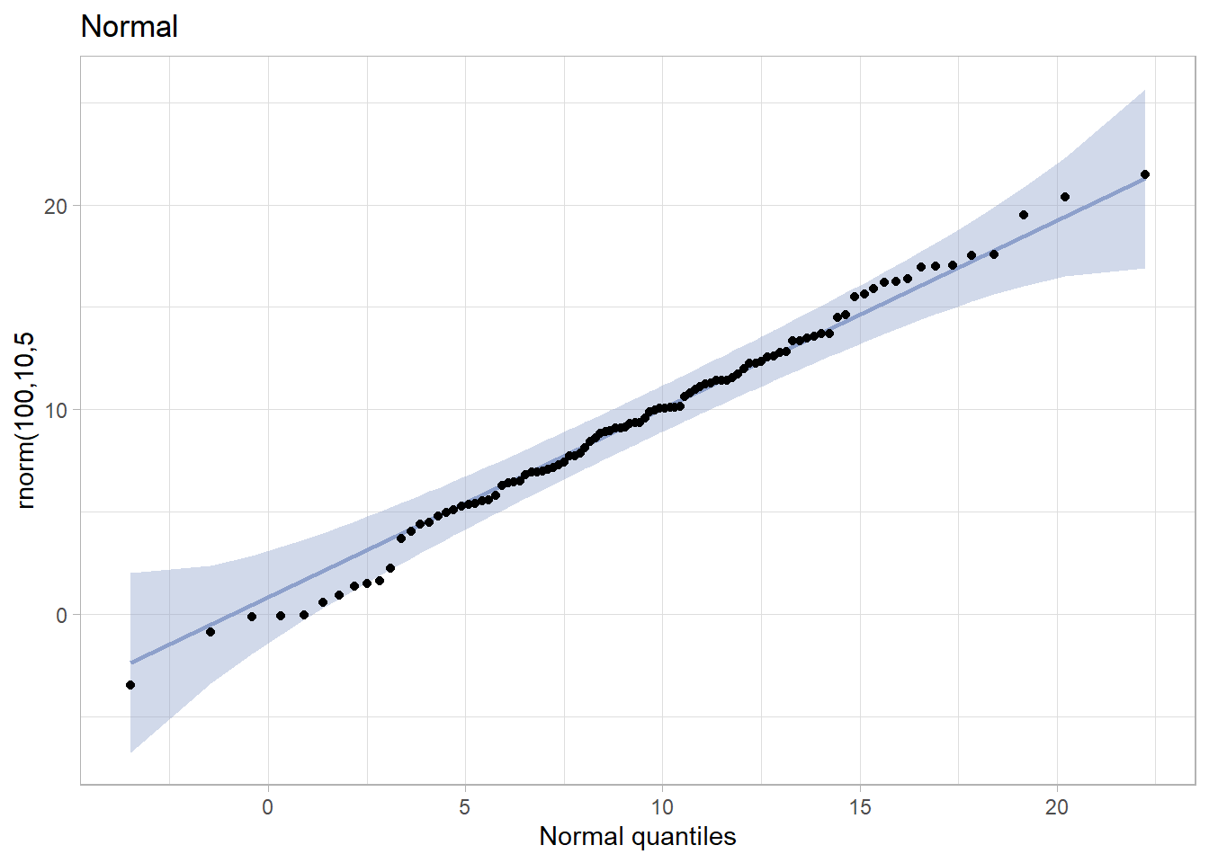
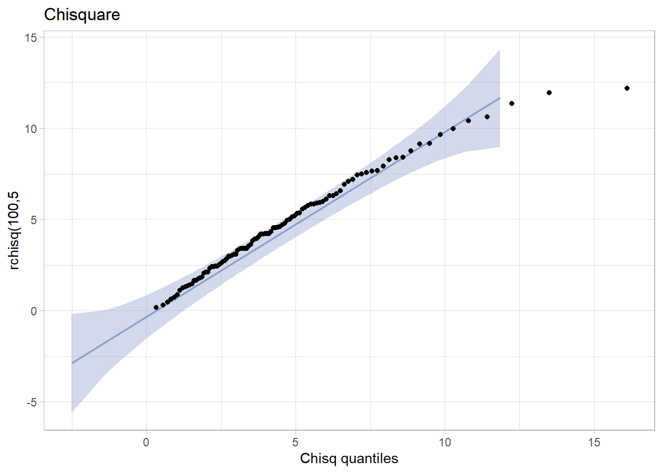
  tibble(x = rchisq(100,5)) %>%
    ggplot(aes(sample = x)) +
    stat_qq_band(bandType = "pointwise", fill = "#8DA0CB", alpha = 0.4) +
    stat_qq_line(colour = "#8DA0CB") +
    stat_qq_point(distribution="chisq") +
    ggtitle("Chisquare") +
    xlab("Chisq quantiles") +
    ylab("rchisq(100,5") +
    theme_light()