Bootstrapping.QMD and its output contain information on how to compute/generate bootstrap samples and compute the bootstrap distribution of a statistic. The various approaches that are presented allow the computation of bias and standard error estimates. In what follows, we make use of the boot package to fit the bootstrap distributions, and from the distribution a number of different confidence intervals for the parameter of interest.
The boot Package’s Bootstrap Distribution
The boot package can be obtained from CRAN. Once loaded, it is easy to use the bootfunction to create bootstrap distributions for a statistic that we have defined. Below we create functions that boot can call.;
Estimate \theta = \mu for N\left(\mu,\, \sigma_0^2\right)
In Rao-Blackwell and Lehmann-Scheffe we saw that it is possible to update a statistic T to make it unbiased. Consider a n random variables X_i \stackrel{iid}{\sim} N(\mu,\, \sigma_0^2) and a statistic T=\sum_{i=1}^n X_i. Since E(T) = n \mu \ne \mu we wish to find an unbiased estimator.
If we let U = X_1 then E(U) = \mu then Rao-Blackwell shows that V = \overline{X} is an unbiased estimator of \mu. To confirm this we can look at the bootstrap distributions of T, U, and V. We start by defining a function that computes the statistics within the boot function.
Code
normal_mystat =function(d, i){ n =length(i) ### Not used and a waste of time T =sum(d[i]) ### Sum_{i=1}^n X_i U = d[i[1]] ### X_1 V =mean(d[i]) ### \overline{X}c(T, U, V) ### Return the list }
We generate a number of observations from a normal distribution of our choice.
Code
### Set the seed to 47 to replicate output. set.seed(47) ### Comment this line out to use the clock. n =100 mu =3 s =5 normal_data =rnorm(n, mu, s)write.csv(normal_data, "normal_data.csv")
We can now use the normal_mystat function to get the bootstrap distributions.
Code
### Use the boot function to run the bootstrap normal_boot =boot(normal_data, normal_mystat, R=9999)### Check the behavior of the statistics normal_boot
Number of bootstrap replications R = 9999
  original   bootBias   bootSE  bootMed
1 325.7445 -0.4233937 48.94685 325.7732
2  12.9735 -9.7014132  4.89544   3.1980
3   3.2574 -0.0042339  0.48947   3.2577
Code
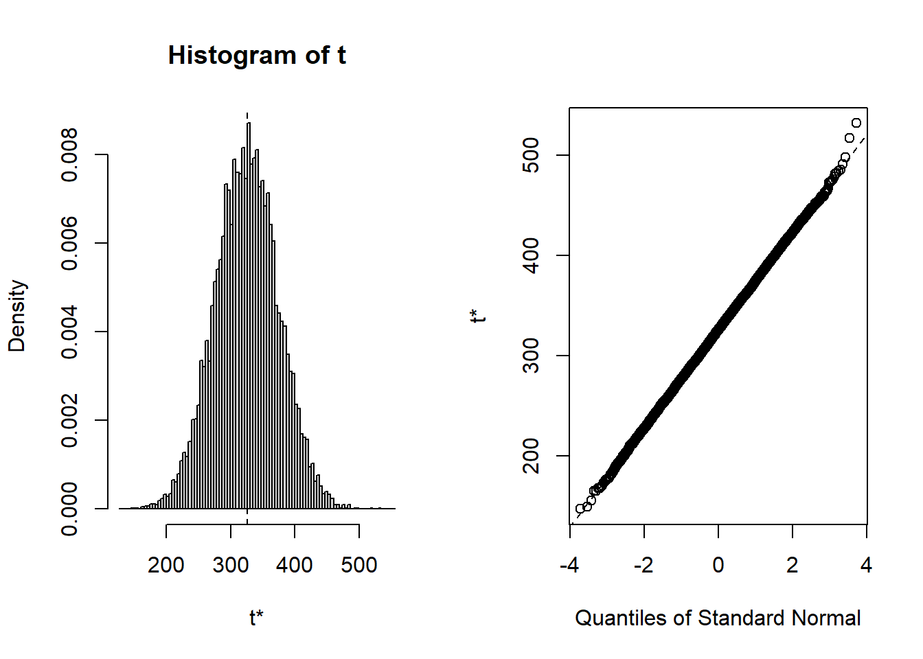
plot(normal_boot)
Code
hist(normal_boot$t[,1])
Code
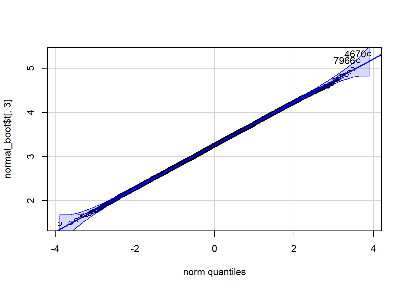
qqPlot(normal_boot$t[,1], distribution="norm")
[1] 4670 7966
Code
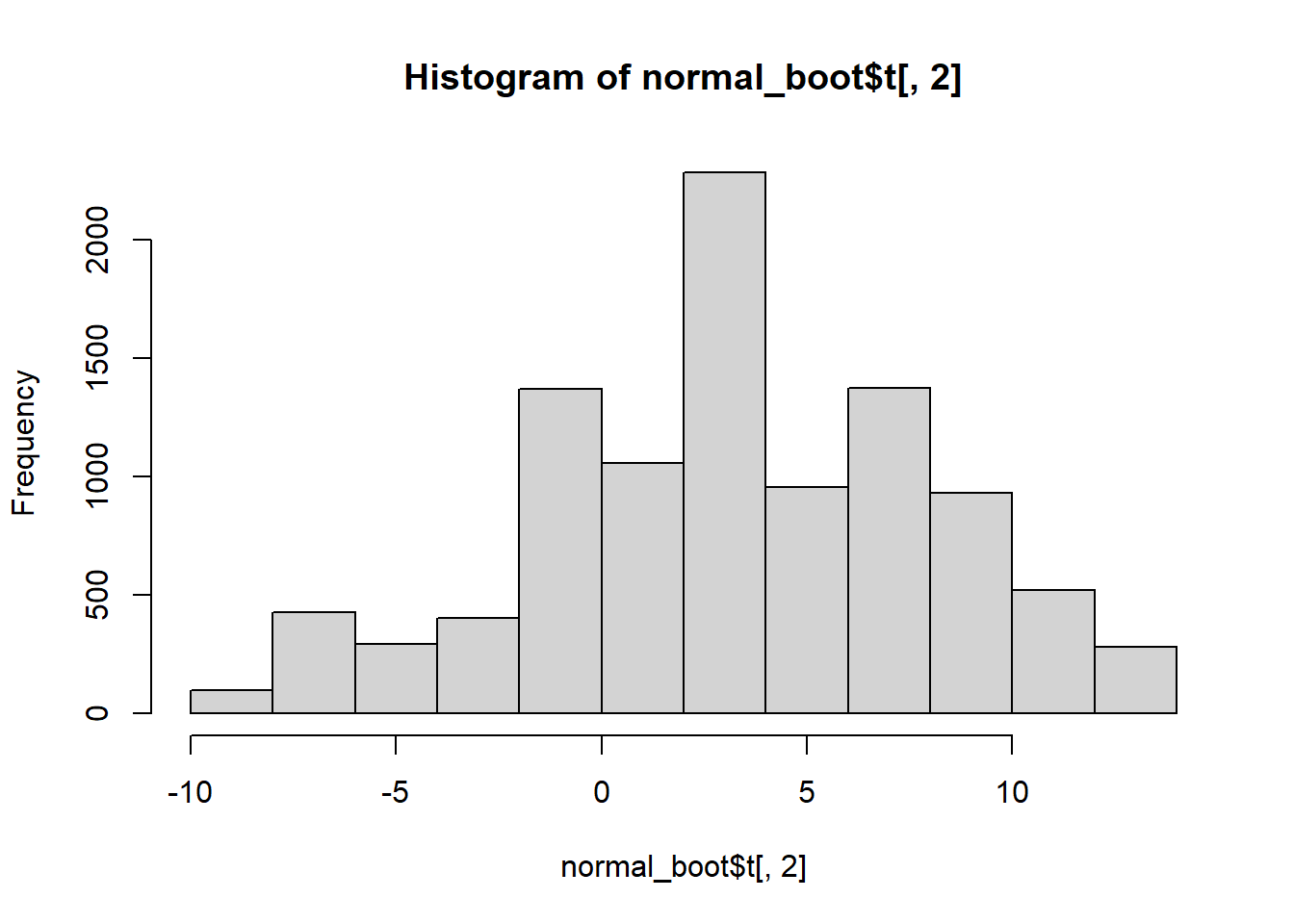
hist(normal_boot$t[,2])
Code
qqPlot(normal_boot$t[,2], distribution="norm")
[1] 12 26
Code
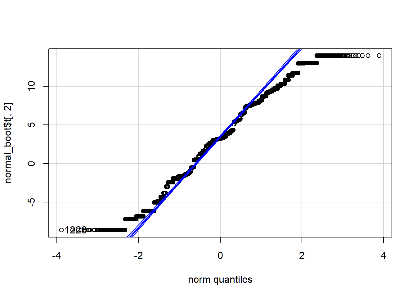
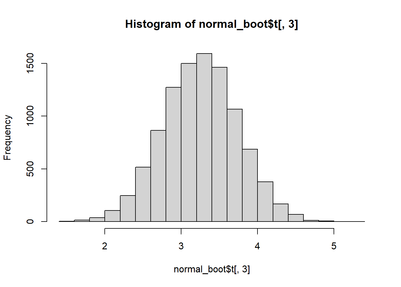
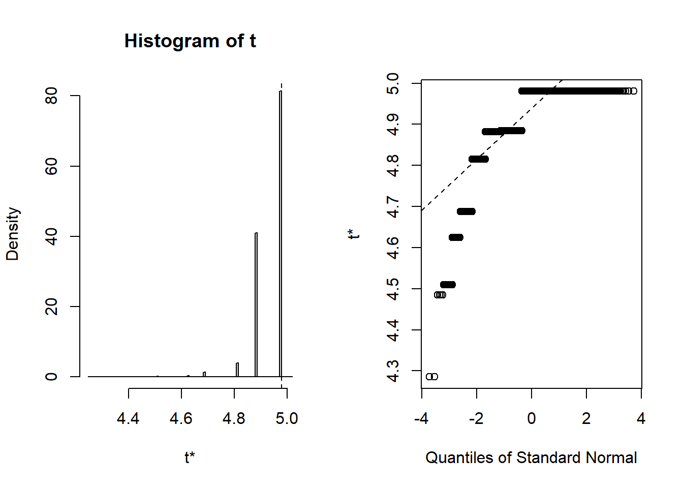
hist(normal_boot$t[,3])
Code
qqPlot(normal_boot$t[,3], distribution="norm")
[1] 4670 7966
Note that the distributions of the sum and mean are both clearly normal. On the other hand, while normal by definition, a single observation appears to be less normal.
Code
quantile(normal_boot$t[,3], c(0.025, 0.975))
    2.5%    97.5%
2.292393 4.205230
Code
args(boot.ci)
function (boot.out, conf = 0.95, type = "all", index = 1L:min(2L,
    length(boot.out$t0)), var.t0 = NULL, var.t = NULL, t0 = NULL,
    t = NULL, L = NULL, h = function(t) t, hdot = function(t) rep(1,
        length(t)), hinv = function(t) t, ...)
NULL
Code
boot.ci(normal_boot, type="all", index=3)
Warning in boot.ci(normal_boot, type = "all", index = 3): bootstrap variances
needed for studentized intervals
BOOTSTRAP CONFIDENCE INTERVAL CALCULATIONS
Based on 9999 bootstrap replicates

CALL :
boot.ci(boot.out = normal_boot, type = "all", index = 3)

Intervals :
Level      Normal              Basic
95%   ( 2.302,  4.221 )   ( 2.310,  4.223 )

Level     Percentile            BCa
95%   ( 2.292,  4.205 )   ( 2.287,  4.200 )
Calculations and Intervals on Original Scale
Code
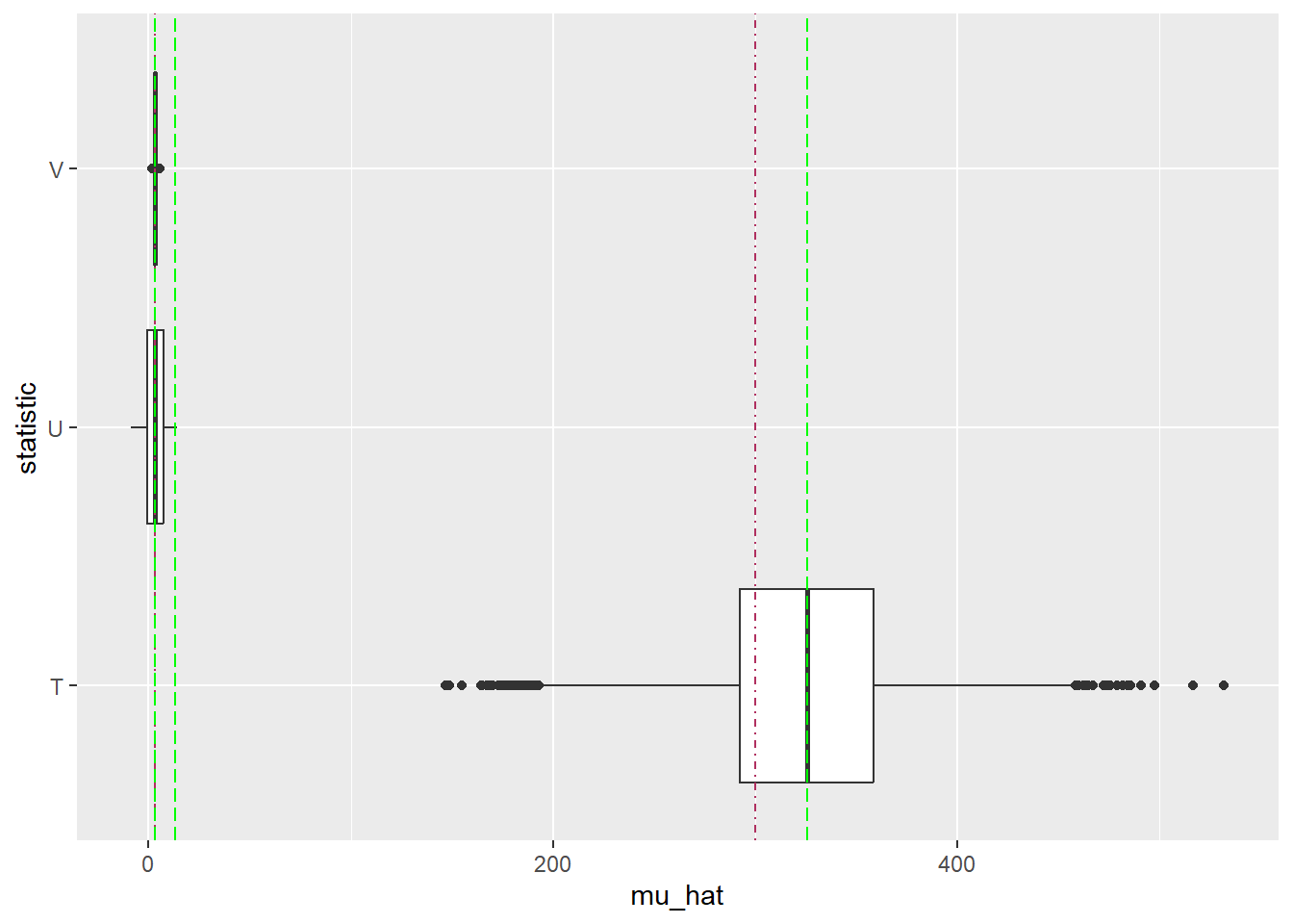
x =as.data.frame(normal_boot$t)colnames(x) =c("T", "U", "V") x |>pivot_longer(cols =c("T","U","V"), names_to ="statistic",values_to ="mu_hat", values_drop_na =TRUE) |>ggplot(aes(y = statistic, x = mu_hat)) +geom_boxplot() +geom_vline(xintercept=c(mu, n*mu), color="maroon", lty=4) +geom_vline(xintercept=c(normal_boot$t0), color="green", lty=5)
We can check that the theoretical and empirical bias and standard errors are similar.
Note that boot.ci uses its own quantile function rather than relying upon the base quantile function. Minor interpolation differences between interval estimates are common.
Estimate \theta for U(0,\theta)
As we saw earlier, Lehmann-Scheffe II can be used to get an estimator for \theta when we have n random variables X_i \stackrel{iid}{\sim} U(0,\, \theta) and a statistic T=X_{[n]}. Since E(T) = n \theta/(n+1) \ne \theta is based upon a minimal sufficient statistic and T can be shown to be complete, we need only to find a constant that makes our new statistic have expectation \theta. We note that V = (n+1)T/n has expectation
E(V) = E\left(\frac{n+1}{n}T\right) = \frac{n+1}{n}\frac{n}{n+1} \theta = \theta
So, V is UMVUE for \theta.
We can check the behavior of the unbiased estimators U = 2 \overline{X} and V = (n+1)X_{[n]}/n using bootstrapping.
Code
uniform_mystat =function(d, i){ n =length(i) ### Require for V T =max(d[i]) ### X_([n]) is biased U =2*mean(d[i]) ### 2 * \overline{X} V = (n+1) * T / n ### (n+1) X_{[n]} / nc(T, U, V) ### Return the list }
We generate a number of observations from a U(0,\, \theta) distribution of our choice.
Code
### Set the seed to 47 to replicate output. set.seed(47) ### Comment this line out to use the clock. n =100 theta =5 uniform_data =runif(n, 0, theta)write.csv(uniform_data, "uniform_data.csv")
We can now use the uniform_mystat function to get the bootstrap distributions.
Code
### Use the boot function to run the bootstrap uniform_boot =boot(uniform_data, uniform_mystat, R=9999)### Check the behavior of the statistics uniform_boot
Number of bootstrap replications R = 9999
  original    bootBias   bootSE bootMed
1   4.9805 -0.04091267 0.062187  4.9805
2   4.7306  0.00075368 0.284215  4.7297
3   5.0303 -0.04132179 0.062809  5.0303
Code
plot(uniform_boot)
Code
hist(uniform_boot$t[,1])
Code
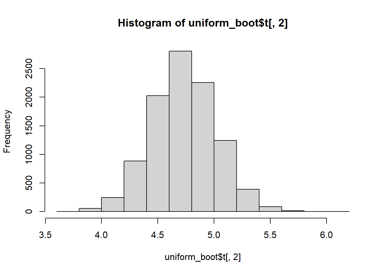
hist(uniform_boot$t[,2])
Code
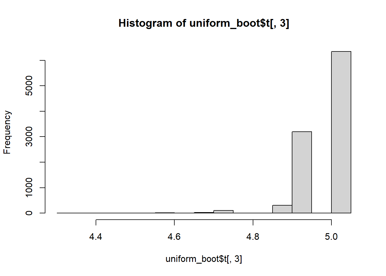
hist(uniform_boot$t[,3])
Note that the distributions of the sum and mean are both clearly normal. On the other hand, while normal by definition, a single observation appears to be less normal.
Code
quantile(uniform_boot$t[,3], c(0.025, 0.975))
    2.5%    97.5%
4.863812 5.030304
Code
args(boot.ci)
function (boot.out, conf = 0.95, type = "all", index = 1L:min(2L,
    length(boot.out$t0)), var.t0 = NULL, var.t = NULL, t0 = NULL,
    t = NULL, L = NULL, h = function(t) t, hdot = function(t) rep(1,
        length(t)), hinv = function(t) t, ...)
NULL
Code
uniform_boot.ci =boot.ci(uniform_boot, index=3)
Warning in boot.ci(uniform_boot, index = 3): bootstrap variances needed for
studentized intervals
Code
uniform_boot.ci
BOOTSTRAP CONFIDENCE INTERVAL CALCULATIONS
Based on 9999 bootstrap replicates

CALL :
boot.ci(boot.out = uniform_boot, index = 3)

Intervals :
Level      Normal              Basic
95%   ( 4.949,  5.195 )   ( 5.030,  5.197 )

Level     Percentile            BCa
95%   ( 4.864,  5.030 )   ( 4.864,  5.030 )
Calculations and Intervals on Original Scale
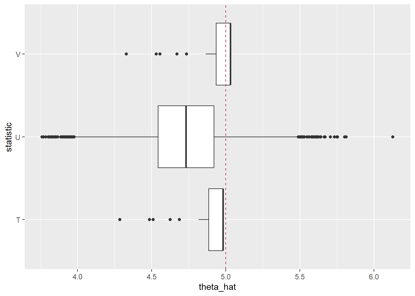
Code
x =as.data.frame(uniform_boot$t)colnames(x) =c("T", "U", "V") x |>pivot_longer(cols =c("T","U","V"), names_to ="statistic",values_to ="theta_hat", values_drop_na =TRUE) |>ggplot(aes(y = statistic, x = theta_hat)) +geom_boxplot() +geom_vline(xintercept=theta, color="maroon", lty=2)