Read Logistic Data

Read Data

The data for the logistic model are stored in a CSV file. We can read the data using either the base or tidyverse functions.

Base

Use read.csv() to get the data. Request a listing of the first six observations as well as a list of the variables.

   retention = read.csv("Data/logistic.csv")

   head(retention)

  STUDID GENDER RACE BDAYMO BDAYYR BEHAVE1 BEHAVE2 ATTEND LETREC1C LETREC1L
1     28      0    2      6     89       1       1      0       23       22
2    139      0    2      5     89       2       2     10       26       24
3    164      1    1      5     89       2       2      0        5        0
4    201      1    2      9     89       1       2      3       21       18
5    221      0    3     12     88       1       1     13        6        4
6    318      1    3     10     89       4       3     17        7        5
  NOREC1 NOREC2 TOTCHILD BRTHORDR BILING ROUND2 RETAINED TEACHER SCHOOL
1     10     12        3        2      0      1        0       2      1
2     20     20        2        1      0      1        0       4      1
3      3      4        2        1      0      1        1       4      1
4     19     20        5        4      0      1        0       2      1
5      2      7        4        3      0      1        1       1      1
6      8     11        3        3      0      1        0       2      1
  LETREC2C LETREC2L AGE1290 RACE1 RACE2 RACE3 RACEO SCHOOL2 TEACHER1 TEACHER2
1       26       25      18     0     1     0     0       0        0        1
2       26       26      19     0     1     0     0       0        0        0
3        5        0      19     1     0     0     0       0        0        0
4       26       22      15     0     1     0     0       0        0        1
5       10        4      24     0     0     1     0       0        1        0
6       19       15      14     0     0     1     0       0        0        1
  TEACHER3 TEACHER4 TOTORDR LR1CRND2 ORDRRND2 TOTCRND2 R2ORDR R2TOT
1        0        0       6       23        2        3      2     3
2        0        1       2       26        1        2      1     2
3        0        1       2        5        1        2      0     0
4        0        0      20       21        4        5      4     5
5        0        0      12        6        3        4      0     0
6        0        0       9        7        3        3      0     0

   names(retention)

 [1] "STUDID"   "GENDER"   "RACE"     "BDAYMO"   "BDAYYR"   "BEHAVE1" 
 [7] "BEHAVE2"  "ATTEND"   "LETREC1C" "LETREC1L" "NOREC1"   "NOREC2"  
[13] "TOTCHILD" "BRTHORDR" "BILING"   "ROUND2"   "RETAINED" "TEACHER" 
[19] "SCHOOL"   "LETREC2C" "LETREC2L" "AGE1290"  "RACE1"    "RACE2"   
[25] "RACE3"    "RACEO"    "SCHOOL2"  "TEACHER1" "TEACHER2" "TEACHER3"
[31] "TEACHER4" "TOTORDR"  "LR1CRND2" "ORDRRND2" "TOTCRND2" "R2ORDR"  
[37] "R2TOT"   

Tidyverse

Use read_csv() to get the data. Again, we request a listing of the first six observations as well as a list of the variables.

   re10tion = read_csv("Data/logistic.csv")

Rows: 111 Columns: 37
── Column specification ────────────────────────────────────────────────────────
Delimiter: ","
dbl (37): STUDID, GENDER, RACE, BDAYMO, BDAYYR, BEHAVE1, BEHAVE2, ATTEND, LE...

ℹ Use `spec()` to retrieve the full column specification for this data.
ℹ Specify the column types or set `show_col_types = FALSE` to quiet this message.

   head(re10tion)

# A tibble: 6 × 37
  STUDID GENDER  RACE BDAYMO BDAYYR BEHAVE1 BEHAVE2 ATTEND LETREC1C LETREC1L
   <dbl>  <dbl> <dbl>  <dbl>  <dbl>   <dbl>   <dbl>  <dbl>    <dbl>    <dbl>
1     28      0     2      6     89       1       1      0       23       22
2    139      0     2      5     89       2       2     10       26       24
3    164      1     1      5     89       2       2      0        5        0
4    201      1     2      9     89       1       2      3       21       18
5    221      0     3     12     88       1       1     13        6        4
6    318      1     3     10     89       4       3     17        7        5
# ℹ 27 more variables: NOREC1 <dbl>, NOREC2 <dbl>, TOTCHILD <dbl>,
#   BRTHORDR <dbl>, BILING <dbl>, ROUND2 <dbl>, RETAINED <dbl>, TEACHER <dbl>,
#   SCHOOL <dbl>, LETREC2C <dbl>, LETREC2L <dbl>, AGE1290 <dbl>, RACE1 <dbl>,
#   RACE2 <dbl>, RACE3 <dbl>, RACEO <dbl>, SCHOOL2 <dbl>, TEACHER1 <dbl>,
#   TEACHER2 <dbl>, TEACHER3 <dbl>, TEACHER4 <dbl>, TOTORDR <dbl>,
#   LR1CRND2 <dbl>, ORDRRND2 <dbl>, TOTCRND2 <dbl>, R2ORDR <dbl>, R2TOT <dbl>

   names(re10tion)

 [1] "STUDID"   "GENDER"   "RACE"     "BDAYMO"   "BDAYYR"   "BEHAVE1" 
 [7] "BEHAVE2"  "ATTEND"   "LETREC1C" "LETREC1L" "NOREC1"   "NOREC2"  
[13] "TOTCHILD" "BRTHORDR" "BILING"   "ROUND2"   "RETAINED" "TEACHER" 
[19] "SCHOOL"   "LETREC2C" "LETREC2L" "AGE1290"  "RACE1"    "RACE2"   
[25] "RACE3"    "RACEO"    "SCHOOL2"  "TEACHER1" "TEACHER2" "TEACHER3"
[31] "TEACHER4" "TOTORDR"  "LR1CRND2" "ORDRRND2" "TOTCRND2" "R2ORDR"  
[37] "R2TOT"   

Change Data Types

Because the data were stored as CSV, the data types of the variables are not necessarily correct. We can re-type the variables before we use them so that R treats them properly.

  retention = re10tion %>%
              mutate(
                Gender = factor(GENDER, 
                                levels = 0:1, 
                                labels = c("Female", "Male") 
                               ),
                Behave1 = factor(BEHAVE1,
                                 levels = 1:4,
                                 labels = c("Good", "Satisfactory", "Unsatisfactory", "Bad"),
                                 ordered = TRUE
                                ),
                Race = factor(RACE,
                              levels = 1:7,
                              labels = c("Black", "White", "Hispanic", "Pacific Islander", 
                                         "Asian", "Filipino", "Other")
                             ),
                Bilingual = factor(BILING,
                                   levels = 0:1,
                                   labels = c("No", "Yes")
                                   ),
                Teacher = factor(TEACHER),
                School = factor(SCHOOL),
                Round_2 = factor(ROUND2, 
                                 levels = 0:1,
                                 labels = c("No", "Yes")
                                 ),
                Retained = factor(RETAINED,
                                  levels = 0:1,
                                  labels = c("No", "Yes")
                                  )
              ) %>%
            rename(
                Student_ID = STUDID,
                Age_12_90 = AGE1290,
                BDay_Mo = BDAYMO,
                BDay_Yr = BDAYYR,
                Let_Rec_1_Cap = LETREC1C,
                Let_Rec_1_Lower = LETREC1L,
                Tot_Children = TOTCHILD,
                Birth_Order = BRTHORDR
                ) %>%
            select(
               Retained,
               Student_ID, Age_12_90, BDay_Mo, BDay_Yr,
               Let_Rec_1_Cap, Let_Rec_1_Lower, Tot_Children,
               Birth_Order, Gender, Behave1, Race,
               Bilingual, Teacher, School, Round_2
              )

  names(retention)

 [1] "Retained"        "Student_ID"      "Age_12_90"       "BDay_Mo"        
 [5] "BDay_Yr"         "Let_Rec_1_Cap"   "Let_Rec_1_Lower" "Tot_Children"   
 [9] "Birth_Order"     "Gender"          "Behave1"         "Race"           
[13] "Bilingual"       "Teacher"         "School"          "Round_2"        

Check the Data

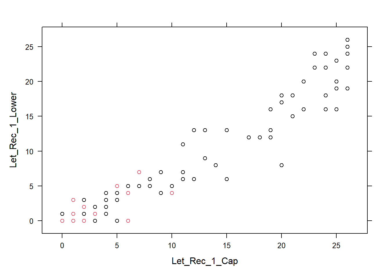
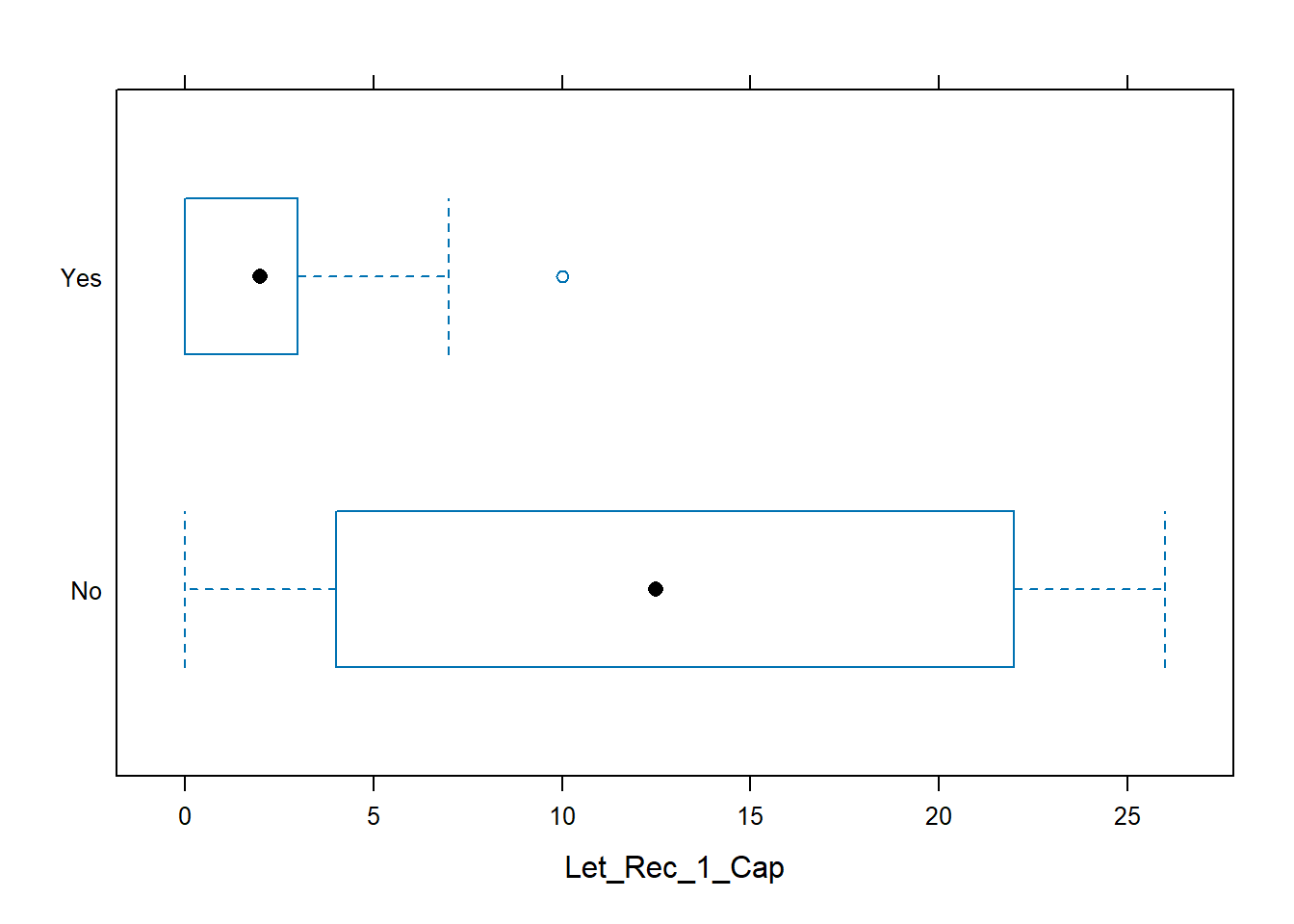
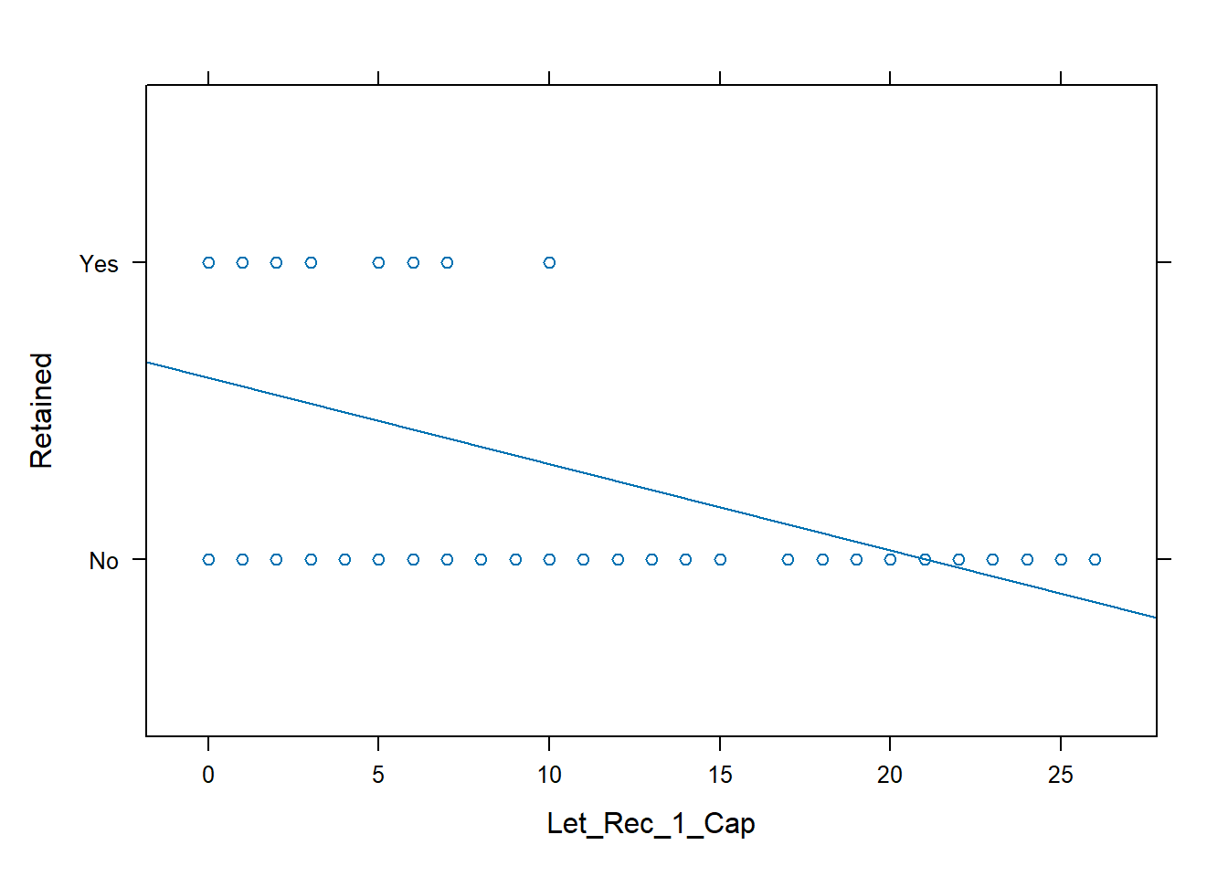
We perform a quick plot or two and a simple logistic model to see if things look okay.

  bwplot(Retained ~ Let_Rec_1_Cap, 
         data=retention
         )

  xyplot(Retained ~ Let_Rec_1_Cap, 
         data=retention, 
         type=c("p","r")
         )

  xyplot(Let_Rec_1_Lower ~ Let_Rec_1_Cap, 
         data=retention, 
         type=c("p"),
         col = retention$Retained
         )

  retained.glm.cap.lower = glm(Retained ~ Let_Rec_1_Cap*Let_Rec_1_Lower, 
                               family = binomial, 
                               data = retention)
  summary(retained.glm.cap.lower)

Call:
glm(formula = Retained ~ Let_Rec_1_Cap * Let_Rec_1_Lower, family = binomial, 
    data = retention)

Coefficients:
                               Estimate Std. Error z value Pr(>|z|)  
(Intercept)                    1.040240   0.465417   2.235   0.0254 *
Let_Rec_1_Cap                 -0.177700   0.178615  -0.995   0.3198  
Let_Rec_1_Lower               -0.199245   0.276776  -0.720   0.4716  
Let_Rec_1_Cap:Let_Rec_1_Lower -0.007099   0.033285  -0.213   0.8311  
---
Signif. codes:  0 '***' 0.001 '**' 0.01 '*' 0.05 '.' 0.1 ' ' 1

(Dispersion parameter for binomial family taken to be 1)

    Null deviance: 141.306  on 110  degrees of freedom
Residual deviance:  86.531  on 107  degrees of freedom
AIC: 94.531

Number of Fisher Scoring iterations: 10

  anova(retained.glm.cap.lower)

Analysis of Deviance Table

Model: binomial, link: logit

Response: Retained

Terms added sequentially (first to last)

                              Df Deviance Resid. Df Resid. Dev  Pr(>Chi)    
NULL                                            110    141.306              
Let_Rec_1_Cap                  1   53.365       109     87.941 2.769e-13 ***
Let_Rec_1_Lower                1    1.356       108     86.585    0.2442    
Let_Rec_1_Cap:Let_Rec_1_Lower  1    0.054       107     86.531    0.8164    
---
Signif. codes:  0 '***' 0.001 '**' 0.01 '*' 0.05 '.' 0.1 ' ' 1

  retained.glm.cap.lower = glm(Retained ~ Let_Rec_1_Cap + Let_Rec_1_Lower,
                               family = binomial, 
                               data = retention)
  summary(retained.glm.cap.lower)

Call:
glm(formula = Retained ~ Let_Rec_1_Cap + Let_Rec_1_Lower, family = binomial, 
    data = retention)

Coefficients:
                Estimate Std. Error z value Pr(>|z|)   
(Intercept)       1.1024     0.3778   2.918  0.00352 **
Let_Rec_1_Cap    -0.1982     0.1513  -1.310  0.19036   
Let_Rec_1_Lower  -0.2392     0.2099  -1.140  0.25444   
---
Signif. codes:  0 '***' 0.001 '**' 0.01 '*' 0.05 '.' 0.1 ' ' 1

(Dispersion parameter for binomial family taken to be 1)

    Null deviance: 141.306  on 110  degrees of freedom
Residual deviance:  86.585  on 108  degrees of freedom
AIC: 92.585

Number of Fisher Scoring iterations: 7

  anova(retained.glm.cap.lower)

Analysis of Deviance Table

Model: binomial, link: logit

Response: Retained

Terms added sequentially (first to last)

                Df Deviance Resid. Df Resid. Dev  Pr(>Chi)    
NULL                              110    141.306              
Let_Rec_1_Cap    1   53.365       109     87.941 2.769e-13 ***
Let_Rec_1_Lower  1    1.356       108     86.585    0.2442    
---
Signif. codes:  0 '***' 0.001 '**' 0.01 '*' 0.05 '.' 0.1 ' ' 1

  retained.glm.cap = glm(Retained ~ Let_Rec_1_Cap, 
                               family = binomial, 
                               data = retention)
  summary(retained.glm.cap)

Call:
glm(formula = Retained ~ Let_Rec_1_Cap, family = binomial, data = retention)

Coefficients:
              Estimate Std. Error z value Pr(>|z|)    
(Intercept)    1.11767    0.37343   2.993  0.00276 ** 
Let_Rec_1_Cap -0.34541    0.08862  -3.898 9.71e-05 ***
---
Signif. codes:  0 '***' 0.001 '**' 0.01 '*' 0.05 '.' 0.1 ' ' 1

(Dispersion parameter for binomial family taken to be 1)

    Null deviance: 141.306  on 110  degrees of freedom
Residual deviance:  87.941  on 109  degrees of freedom
AIC: 91.941

Number of Fisher Scoring iterations: 7

  anova(retained.glm.cap)

Analysis of Deviance Table

Model: binomial, link: logit

Response: Retained

Terms added sequentially (first to last)

              Df Deviance Resid. Df Resid. Dev  Pr(>Chi)    
NULL                            110    141.306              
Let_Rec_1_Cap  1   53.365       109     87.941 2.769e-13 ***
---
Signif. codes:  0 '***' 0.001 '**' 0.01 '*' 0.05 '.' 0.1 ' ' 1