  x <- c(3, 4, 4, 5, 6, 6)
  y <- c(3, 3, 4, 6, 5, 7)
  sixpts <- data.frame(x,y)
  sixpts
x y
1 3 3
2 4 3
3 4 4
4 5 6
5 6 5
6 6 7The six point example uses six data points. Yes, it is small and boring.
x <- c(3, 4, 4, 5, 6, 6)
y <- c(3, 3, 4, 6, 5, 7)
sixpts <- data.frame(x,y)
sixpts x y
1 3 3
2 4 3
3 4 4
4 5 6
5 6 5
6 6 7The points can be plotted.
  p_load(ggplot2)
  p = ggplot(sixpts, aes(x = x, y = y)) +
    geom_point() +
    theme_bw() +  # Add theme for cleaner look
    coord_cartesian(xlim = c(0,7), ylim=c(-1,8))+
    annotate(geom="segment", y=seq(-1,8,0.25), yend = seq(-1,8,0.25), x=-0.25, xend=7.25, col="lightgrey") +
    annotate(geom="segment", x=seq(-0.25,7.25,0.25), xend = seq(-0.25,7.25,0.25), y=-1, yend=8, col="lightgrey")
  p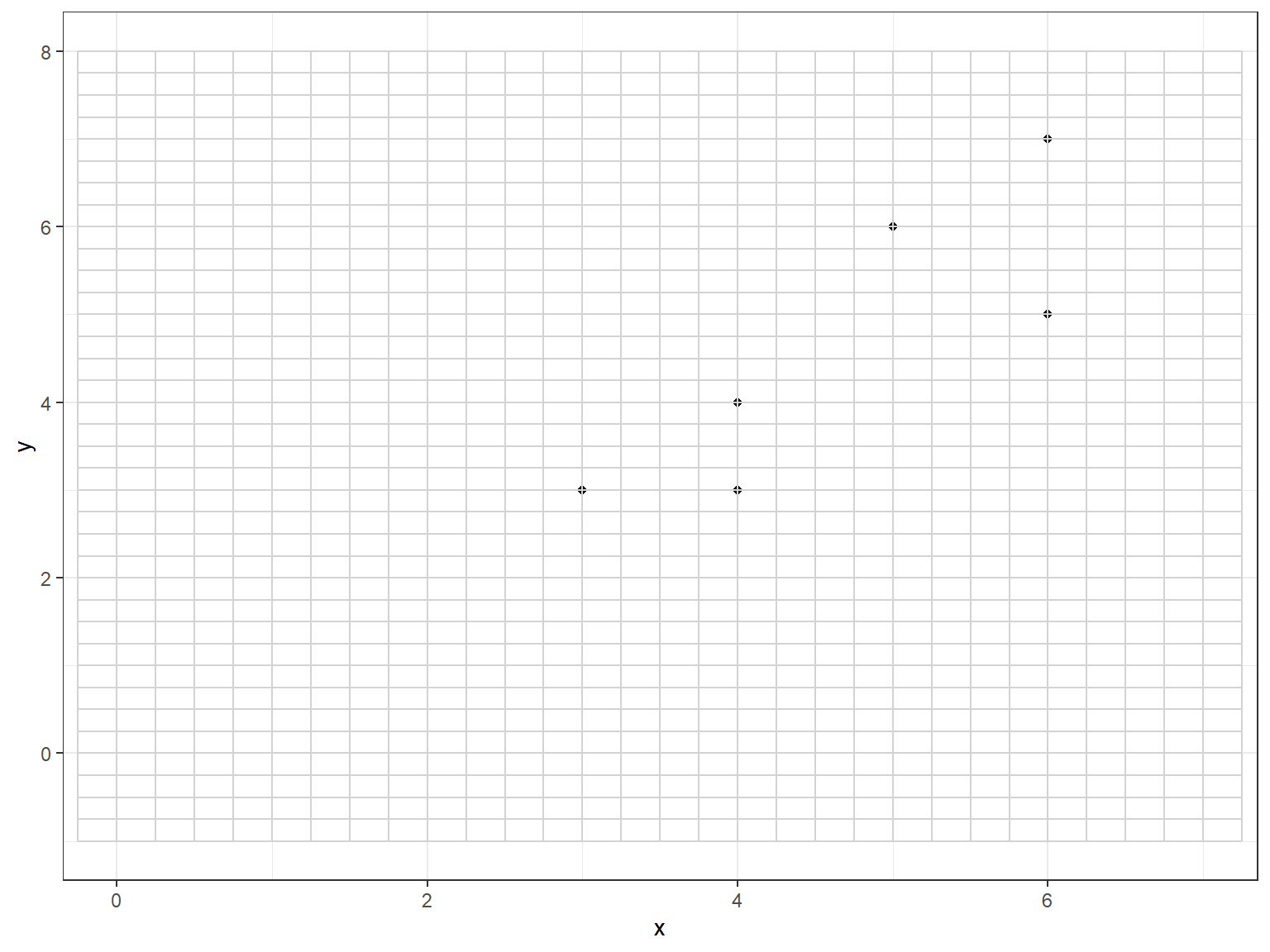
  pdf("Six_Points.pdf")
    p
  dev.off()
png
2 The “best fit” linear regression line can be added.
  p = ggplot(sixpts, aes(x = x, y = y)) +
    geom_smooth(method = "lm", se = FALSE, color = "darkgrey") +  # Plot regression slope
    geom_point() +
    theme_bw() +  # Add theme for cleaner look
    coord_cartesian(xlim = c(0,7), ylim=c(-1,8))
  p
`geom_smooth()` using formula = 'y ~ x'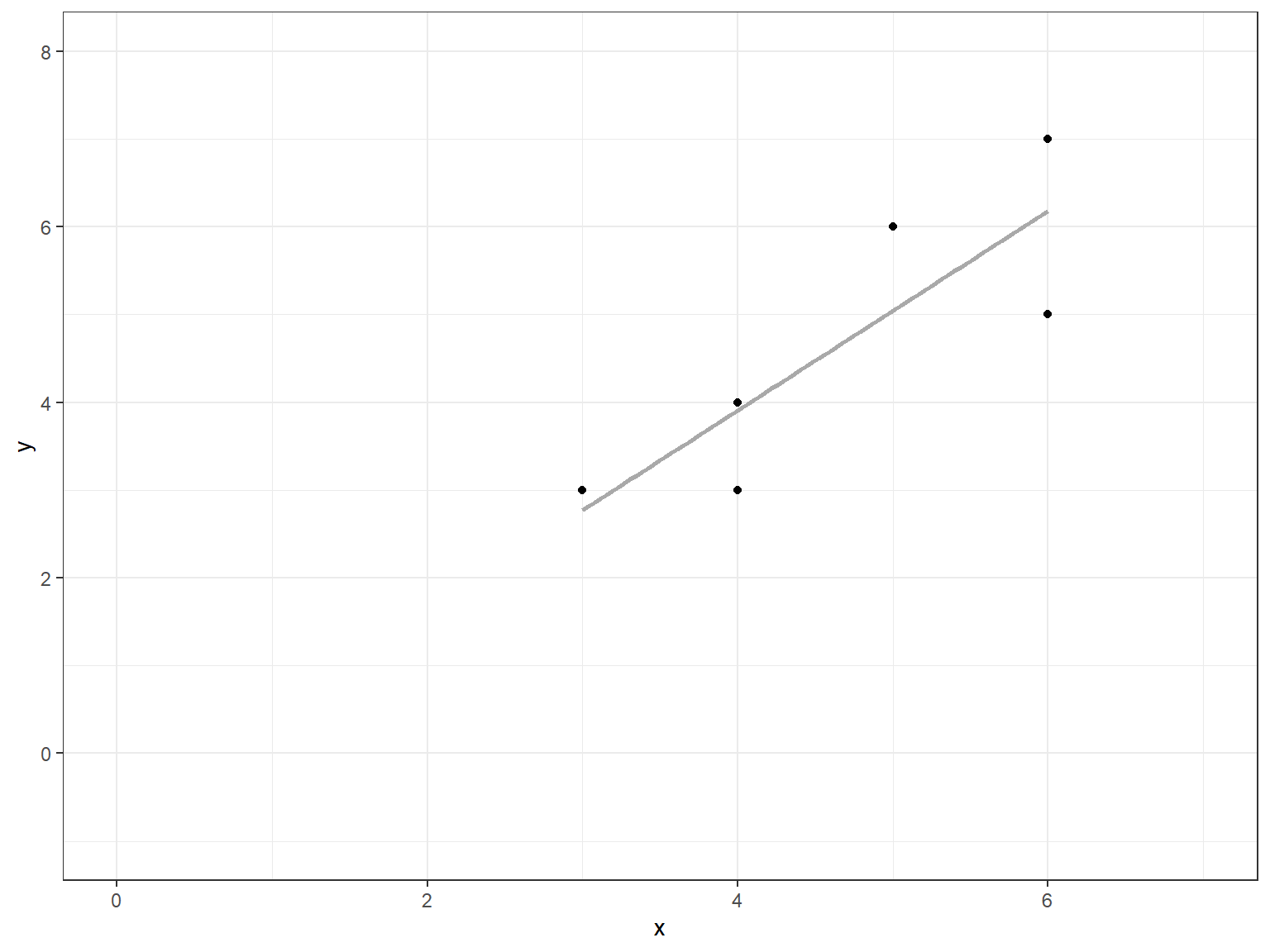
  pdf("Six_Points_Reg.pdf")
    p
`geom_smooth()` using formula = 'y ~ x' dev.off()png
2 The vertical errors (residuals) can be observed.
  sixpts$predicted <- predict(lm(y~x, data=sixpts))
  p = ggplot(sixpts, aes(x = x, y = y)) +
    geom_smooth(method = "lm", se = FALSE, color = "darkgrey") +  # Plot regression slope
    geom_segment(aes(xend = x, yend = predicted), alpha = .2) + # alpha to fade lines
    geom_point() +
    geom_point(aes(y = predicted), shape = 1) +
    theme_bw() +  # Add theme for cleaner look
    coord_cartesian(xlim = c(0,7), ylim=c(-1,8))

   p
`geom_smooth()` using formula = 'y ~ x'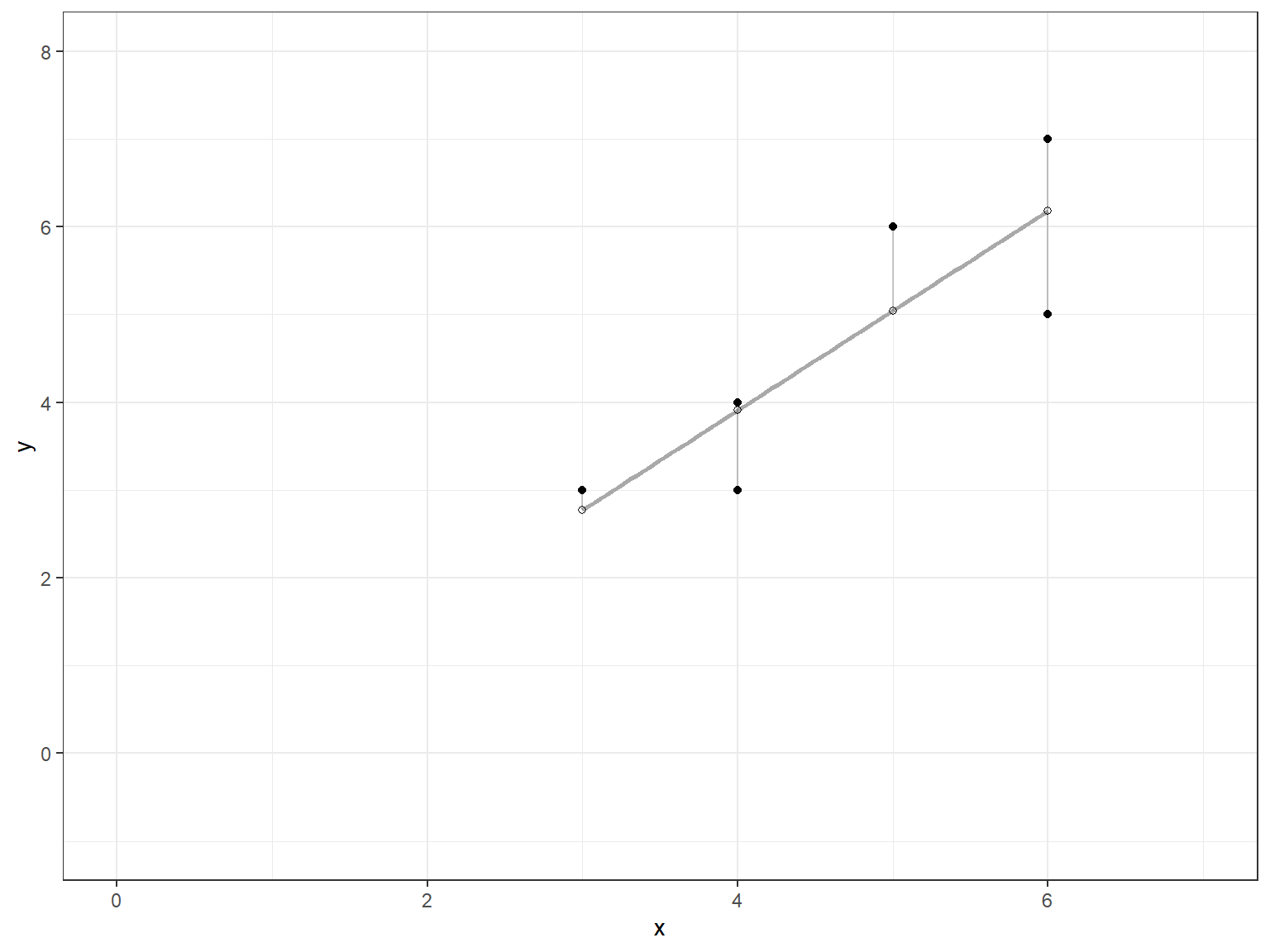
  pdf("Six_Points_Resid.pdf")
    p
`geom_smooth()` using formula = 'y ~ x' dev.off()png
2 We now show that the regression line goes through (\bar{x},\ \bar{y}) = (4.6667, 4.6667).
   p = ggplot(sixpts, aes(x = x, y = y)) +
    geom_smooth(method = "lm", se = FALSE, color = "darkgrey") +  # Plot regression slope
    geom_segment(aes(xend = x, yend = predicted), alpha = .2) + # alpha to fade lines
    geom_point() +
    geom_point(aes(y = predicted), shape = 1) +
    theme_bw() +  # Add theme for cleaner look
    geom_hline(yintercept=mean(y), lty = 3, col = 1) +
    geom_vline(xintercept=mean(x), lty = 3, col = 1) +
    coord_cartesian(xlim = c(0,7), ylim=c(-1,8))
  p
`geom_smooth()` using formula = 'y ~ x'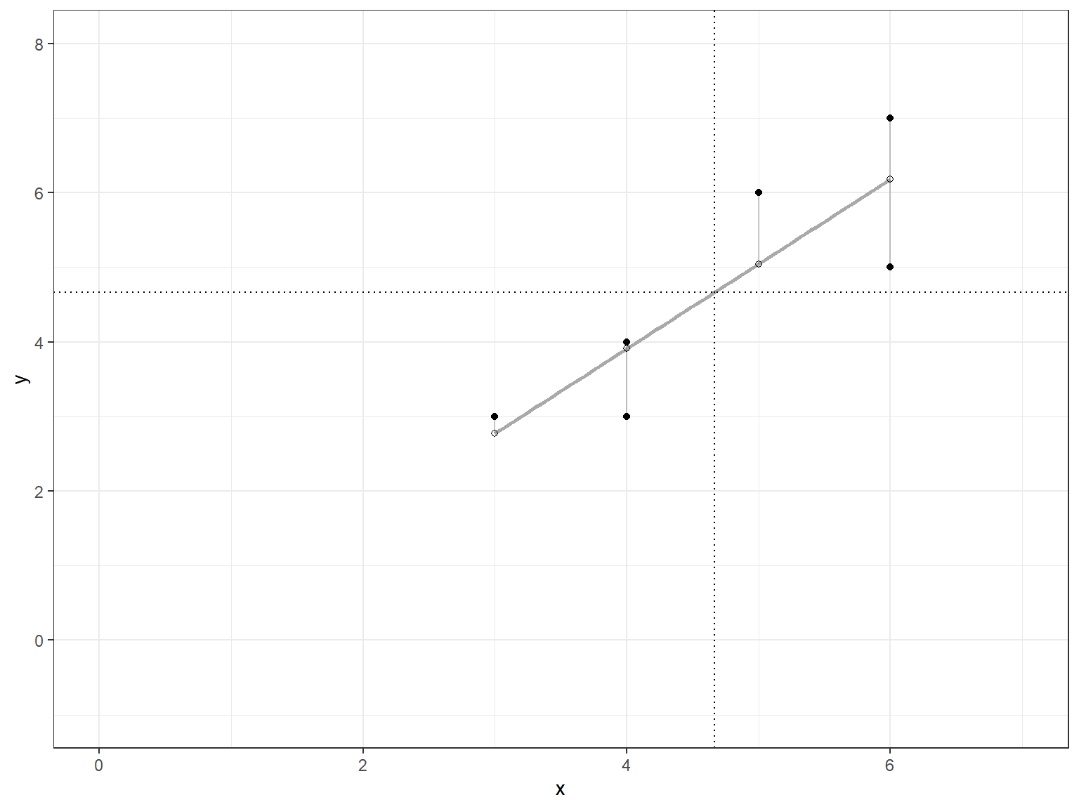
  pdf("Six_Points_Reg_Resid.pdf")
    p
`geom_smooth()` using formula = 'y ~ x' dev.off()png
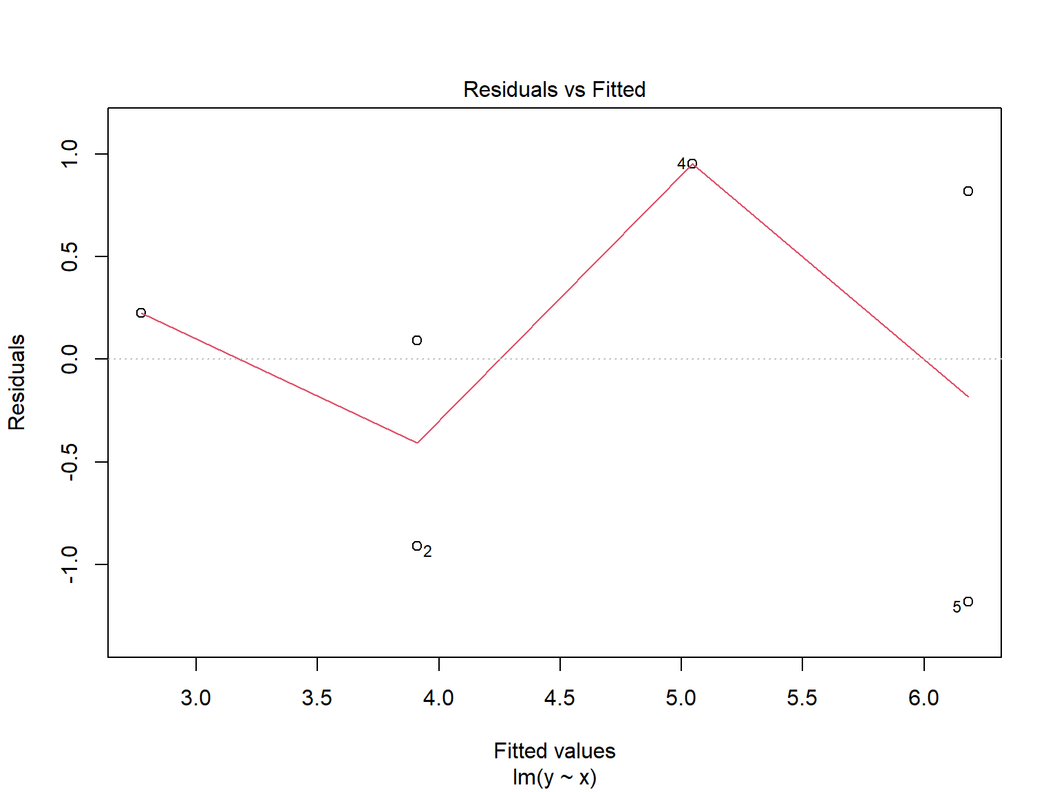
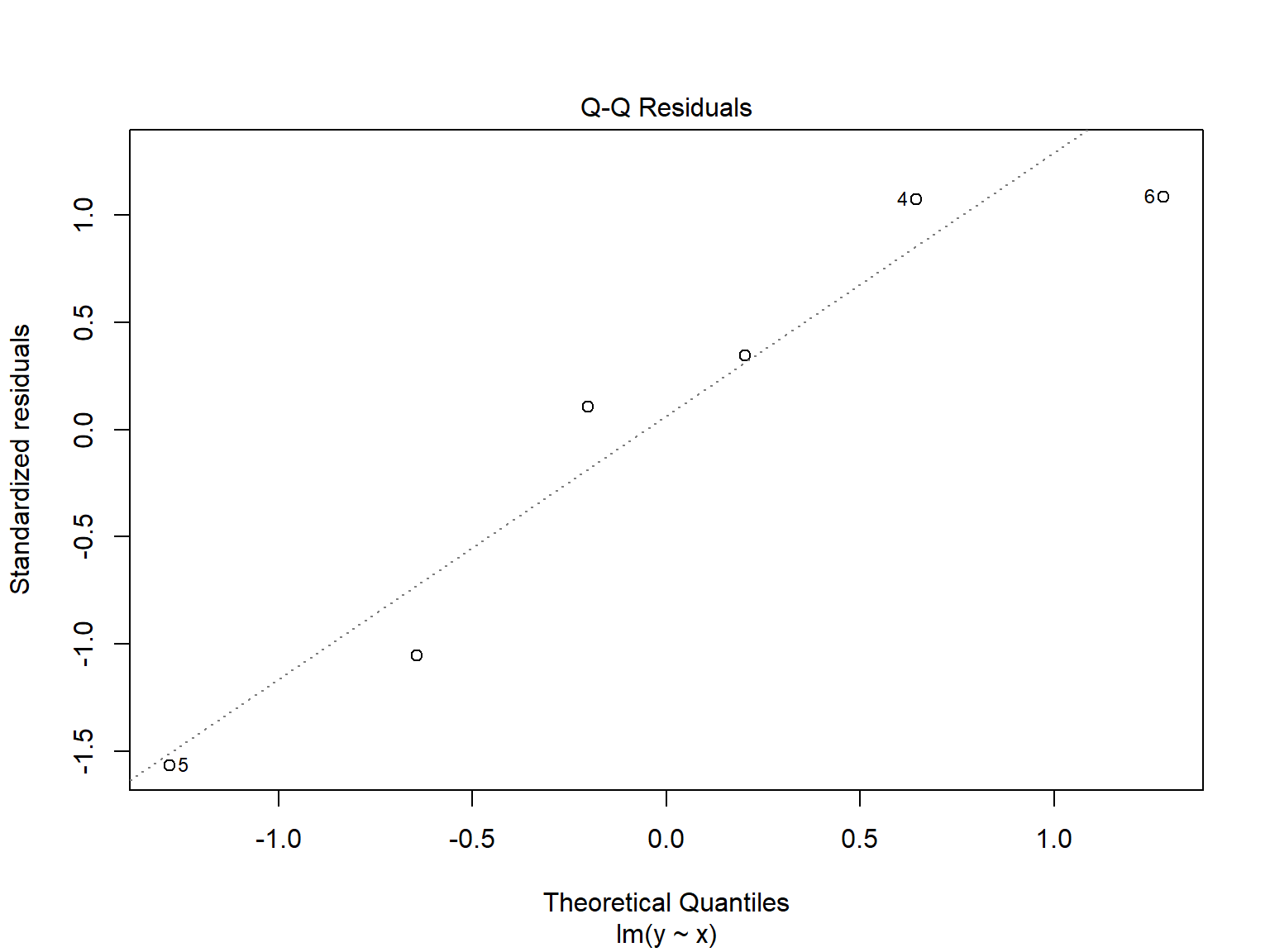
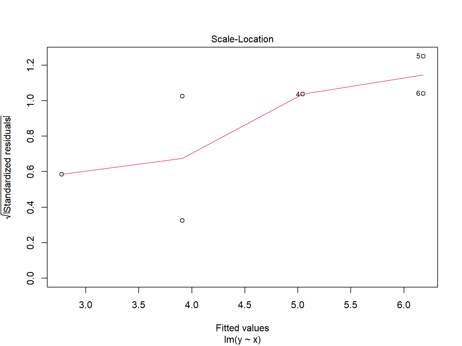
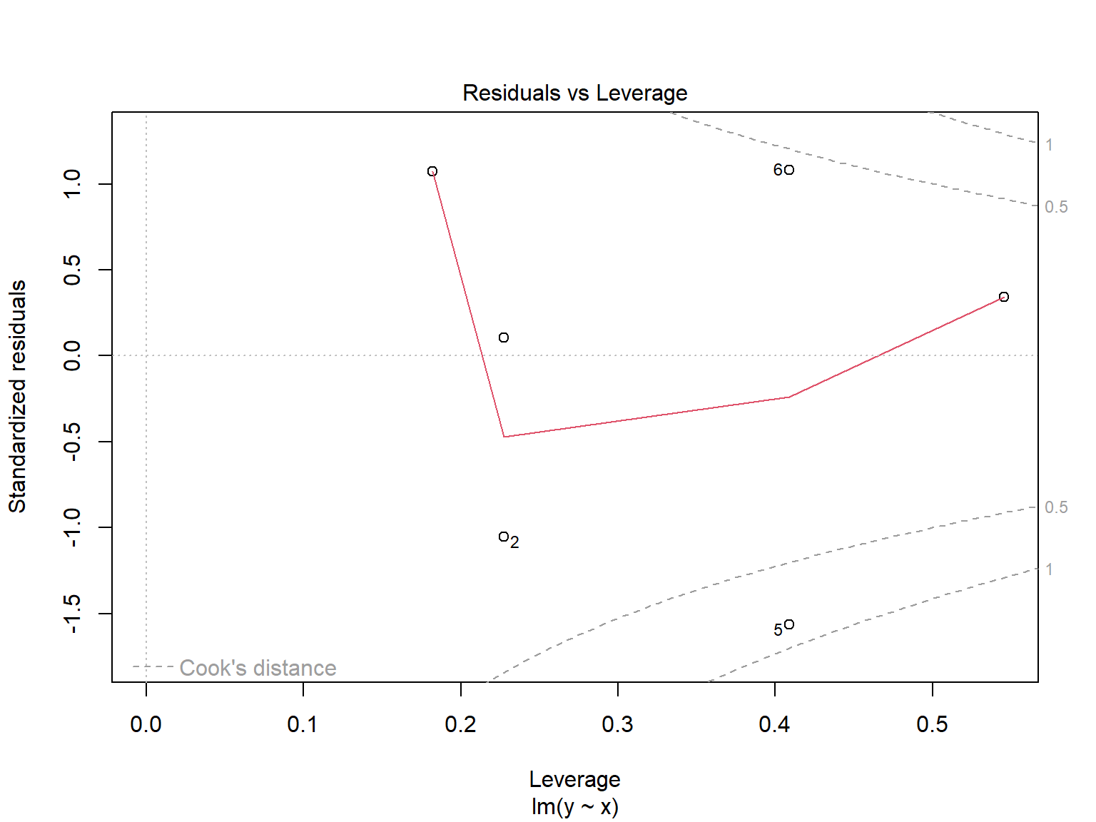
2 We now fit the regression model and look at its characteristics.
  lm.y.x = lm(y ~ x, data=sixpts)
  lm.y.x
Call:
lm(formula = y ~ x, data = sixpts)

Coefficients:
(Intercept)            x
-0.6364 1.1364 summary(lm.y.x)
Call:
lm(formula = y ~ x, data = sixpts)

Residuals:
       1        2        3        4        5        6
 0.22727 -0.90909  0.09091  0.95455 -1.18182  0.81818

Coefficients:
            Estimate Std. Error t value Pr(>|t|)
(Intercept)  -0.6364     1.7405  -0.366   0.7332
x             1.1364     0.3629   3.131   0.0351 *
---
Signif. codes:  0 '***' 0.001 '**' 0.01 '*' 0.05 '.' 0.1 ' ' 1

Residual standard error: 0.9828 on 4 degrees of freedom
Multiple R-squared:  0.7102,    Adjusted R-squared:  0.6378
F-statistic: 9.804 on 1 and 4 DF, p-value: 0.03515 anova(lm.y.x)Analysis of Variance Table
Response: y
Df Sum Sq Mean Sq F value Pr(>F)
x 1 9.4697 9.4697 9.8039 0.03515 *
Residuals 4 3.8636 0.9659
---
Signif. codes: 0 '***' 0.001 '**' 0.01 '*' 0.05 '.' 0.1 ' ' 1 plot(lm.y.x)